Stan の data ブロックと parameters ブロックを入れ替える

偉大なるごみ箱師のスライド data ブロックと parameters ブロックの関係 を試したくなったので、Kosugitti 先生の 世界一簡単なrstanコード でやってみる。

inf_params.stan

######################################## パラメータ推定のための Stan コード
data{
  int<lower=0> N;
  real x[N];
}

parameters {
  real mu;
  real<lower=0> s;
}

model{
  x ~ normal(mu, s);
  mu ~ normal(0, 100);
  s ~ inv_gamma(0.001, 0.001);
}

R

######################################## 普通に Stan を実行してパラメータ推定
library(rstan)

set.seed(123)

N <- 1000
x <- rnorm(N, mean=0, sd=1)

n.iter <- 1000
n.chains <- 4
datastan <- list(N=N, x=x)
fit <- stan(file="inf_params.stan", data=datastan, iter=n.iter, chain=n.chains)
traceplot(fit, ask=FALSE)
print(fit, digit=3)

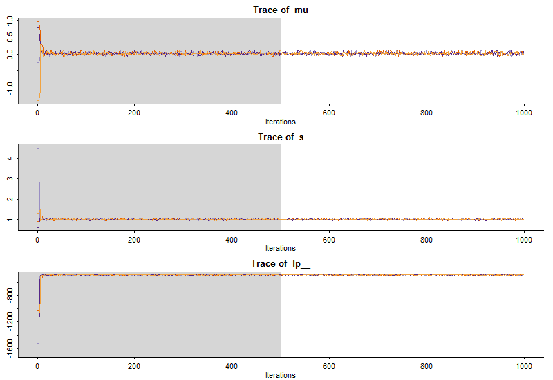
結果

         mean se_mean    sd     2.5%      25%      50%      75%    97.5% n_eff  Rhat
mu      0.017   0.001 0.033   -0.049   -0.004    0.017    0.038    0.083  1233 0.999
s       0.993   0.001 0.022    0.952    0.977    0.992    1.007    1.038  1365 1.000
lp__ -492.187   0.040 1.032 -494.824 -492.604 -491.850 -491.451 -491.181   673 1.000

R

######################################## 推定されたパラメータを取得
library(foreach)
params <- foreach(i = seq_len(n.chains), .combine=rbind) %do% {
  reject <- seq_len(fit@sim$warmup)
  with(fit@sim$samples[[i]], 
    data.frame(mu=mu[-reject], s=s[-reject])
  )
}

skeleton <- list(mu=0, s=0)
param.list <- relist(as.relistable(colMeans(params)), skeleton)
print(param.list)

結果

$mu
[1] 0.01694555
$s
[1] 0.9929771

sampling.stan

######################################## サンプリングのための Stan コード
data{
  real mu;
  real<lower=0> s;
}

parameters {
  real x;
}

model{
  x ~ normal(mu, s);
}

R

######################################## Stan でサンプリング
fit2 <- stan(file="sampling.stan", data=param.list, iter=n.iter, chain=n.chains)
traceplot(fit2, ask=FALSE)
print(fit2, digit=3)

結果

       mean se_mean    sd   2.5%    25%    50%    75%  97.5% n_eff  Rhat
x     0.082   0.040 0.992 -1.856 -0.540  0.124  0.719  1.955   622 1.001
lp__ -0.501   0.023 0.707 -2.361 -0.701 -0.203 -0.044 -0.001   930 1.004

R

######################################## サンプリング結果を格納
x.res <- fit2@sim$samples[[1]]$x
data <- rbind(data.frame(x=x, type="x"), data.frame(x=x.res, type="x.res"))

R

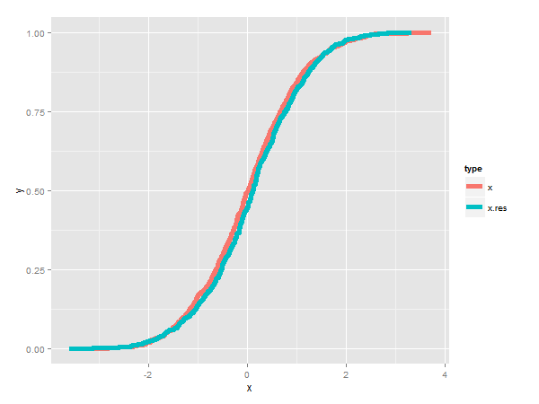
######################################## 経験分布関数の描画
library(ggplot2)
ggplot(data, aes(x=x, color=type)) + stat_ecdf(size=2)

R

######################################## Q-Q プロットの描画
qqplot(x, x.res)
abline(0, 1, col=2, lwd=2)

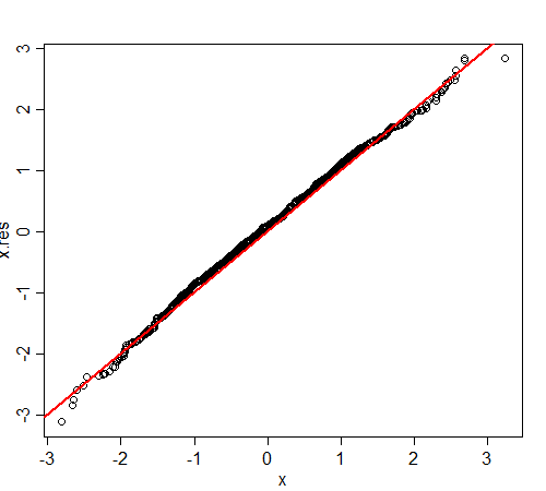
R

######################################## コルモゴロフ-スミルノフ検定
ks.test(x, x.res)

結果

    Two-sample Kolmogorov-Smirnov test

data:  x and x.res
D = 0.059, p-value = 0.06155
alternative hypothesis: two-sided