Q. 散布図と周辺分布をあわせて描きたいです。
-
{ggExtra}パッケージのggMarginal関数は見た目がイマイチです。 -
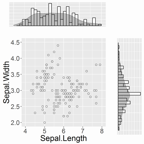
{gridExtra}パッケージのgrid.arrange関数を使うと以下のようになってしまい、軸の目盛が揃わなくて困っています。
library(ggplot2)

p_xy <- ggplot(iris, aes(Sepal.Length, Sepal.Width)) +
  theme(text=element_text(size=20)) +
  geom_point(alpha=0.8, size=2, shape=1) +
  scale_x_continuous(limits=c(4, 8)) +
  scale_y_continuous(limits=c(2, 4.5))

p_x <- ggplot(iris, aes(Sepal.Length)) +
  theme(axis.text.x=element_blank(), axis.text.y=element_blank(), axis.ticks=element_blank()) +
  geom_histogram(aes(y=..density..), colour='black', fill='white') +
  geom_density(alpha=0.3, fill='gray20') +
  scale_x_continuous(limits=c(4, 8)) +
  labs(x='', y='')

p_y <- ggplot(iris, aes(Sepal.Width)) +
  theme(axis.text.x=element_blank(), axis.text.y=element_blank(), axis.ticks=element_blank()) +
  coord_flip() +
  geom_histogram(aes(y=..density..), colour='black', fill='white') +
  geom_density(alpha=0.3, fill='gray20') +
  scale_x_continuous(limits=c(2, 4.5)) +
  labs(x='', y='')


library(gridExtra)
png(file='NG_example.png', res=300, w=1500, h=1500)
grid.arrange(
  arrangeGrob(p_x,       ncol=2, widths=c(3,1)),
  arrangeGrob(p_xy, p_y, ncol=2, widths=c(3,1)),
  heights=c(1,3)
)
dev.off()
A.
{ggplot2}パッケージのtheme関数のplot.marginオプションを手調整で頑張る方法があります。
http://stackoverflow.com/questions/8545035/scatterplot-with-marginal-histograms-in-ggplot2
しかし、この方法は手調整が大変でやってられません。そこで{gtable}パッケージを使います。基本的な使い方はbaptisteさんが以下で説明しています。
https://github.com/baptiste/gridextra/wiki/arranging-ggplot
library(ggplot2)
p_xy <- ggplot(iris, aes(Sepal.Length, Sepal.Width)) +
theme(text=element_text(size=20)) +
geom_point(alpha=0.8, size=2, shape=1) +
scale_x_continuous(limits=c(4, 8)) +
scale_y_continuous(limits=c(2, 4.5))
p_x <- ggplot(iris, aes(Sepal.Length)) +
theme(axis.text.x=element_blank(), axis.text.y=element_blank(), axis.ticks=element_blank()) +
geom_histogram(aes(y=..density..), colour='black', fill='white') +
geom_density(alpha=0.3, fill='gray20') +
scale_x_continuous(limits=c(4, 8)) +
labs(x='', y='')
p_y <- ggplot(iris, aes(Sepal.Width)) +
theme(axis.text.x=element_blank(), axis.text.y=element_blank(), axis.ticks=element_blank()) +
coord_flip() +
geom_histogram(aes(y=..density..), colour='black', fill='white') +
geom_density(alpha=0.3, fill='gray20') +
scale_x_continuous(limits=c(2, 4.5)) +
labs(x='', y='')
p_emp <- ggplot(data.frame(0,0)) + theme_bw() + theme(rect=element_rect(fill='white'), panel.border=element_blank())
g_xy <- ggplotGrob(p_xy)
g_x <- ggplotGrob(p_x)
g_y <- ggplotGrob(p_y)
g_emp <- ggplotGrob(p_emp)
g1 <- cbind(g_x, g_emp, size='first')
g2 <- cbind(g_xy, g_y, size='first')
g <- rbind(g1, g2, size='first')
g$widths[1:3] <- grid::unit.pmax(g1$widths[1:3], g2$widths[1:3])
g$heights[7:12] <- g$widths[5:10] <- rep(unit(0.3,'mm'), 6)
g$heights[6] <- g$widths[11] <- unit(3,'cm')
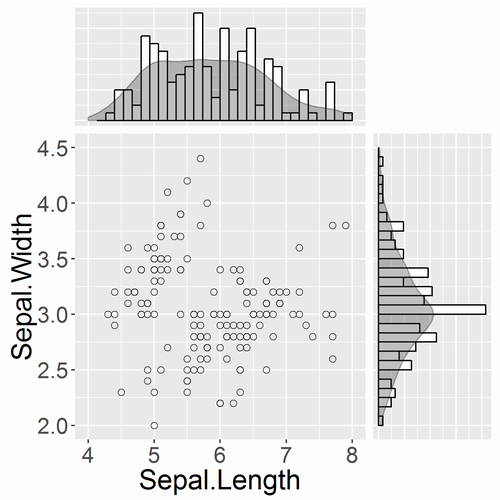
png(file='OK_example.png', res=300, w=1500, h=1500)
grid::grid.draw(g)
dev.off()
コードの説明
基本的な方針はggplotGrob関数で個々のplotからgrob(graphical objectとのことです)を作り、それをrbindとcbindで組み合わせていきます。上記ではcbind関数のsizeオプションは'first'にしていますが、デフォルトの'max'や'min'ではエラーが出てしまいます(既知のバグのようです)。
上記のgtableクラスのオブジェクトであるgをprintしますと以下になっています。
> g
TableGrob (20 x 14) "layout": 68 grobs
    z         cells       name                                   grob
1   0 ( 1-10, 1- 7) background        rect[plot.background..rect.339]
2   5 ( 5- 5, 3- 3)     spacer                         zeroGrob[NULL]
3   7 ( 6- 6, 3- 3)     axis-l    absoluteGrob[GRID.absoluteGrob.334]
4   3 ( 7- 7, 3- 3)     spacer                         zeroGrob[NULL]
5   6 ( 5- 5, 4- 4)     axis-t                         zeroGrob[NULL]
6   1 ( 6- 6, 4- 4)      panel               gTree[panel-1.gTree.320]
7   9 ( 7- 7, 4- 4)     axis-b    absoluteGrob[GRID.absoluteGrob.330]
8   4 ( 5- 5, 5- 5)     spacer                         zeroGrob[NULL]
9   8 ( 6- 6, 5- 5)     axis-r                         zeroGrob[NULL]
10  2 ( 7- 7, 5- 5)     spacer                         zeroGrob[NULL]
11 10 ( 4- 4, 4- 4)     xlab-t                         zeroGrob[NULL]
12 11 ( 8- 8, 4- 4)     xlab-b titleGrob[axis.title.x..titleGrob.323]
13 12 ( 6- 6, 2- 2)     ylab-l titleGrob[axis.title.y..titleGrob.326]
14 13 ( 6- 6, 6- 6)     ylab-r                         zeroGrob[NULL]
15 14 ( 3- 3, 4- 4)   subtitle  zeroGrob[plot.subtitle..zeroGrob.336]
16 15 ( 2- 2, 4- 4)      title     zeroGrob[plot.title..zeroGrob.335]
17 16 ( 9- 9, 4- 4)    caption   zeroGrob[plot.caption..zeroGrob.337]
18  0 ( 1-10, 8-14) background        rect[plot.background..rect.392]
19  5 ( 5- 5,10-10)     spacer                         zeroGrob[NULL]
20  7 ( 6- 6,10-10)     axis-l                         zeroGrob[NULL]
21  3 ( 7- 7,10-10)     spacer                         zeroGrob[NULL]
22  6 ( 5- 5,11-11)     axis-t                         zeroGrob[NULL]
23  1 ( 6- 6,11-11)      panel               gTree[panel-1.gTree.387]
24  9 ( 7- 7,11-11)     axis-b                         zeroGrob[NULL]
25  4 ( 5- 5,12-12)     spacer                         zeroGrob[NULL]
26  8 ( 6- 6,12-12)     axis-r                         zeroGrob[NULL]
27  2 ( 7- 7,12-12)     spacer                         zeroGrob[NULL]
28 10 ( 4- 4,11-11)     xlab-t                         zeroGrob[NULL]
29 11 ( 8- 8,11-11)     xlab-b                         zeroGrob[NULL]
30 12 ( 6- 6, 9- 9)     ylab-l                         zeroGrob[NULL]
31 13 ( 6- 6,13-13)     ylab-r                         zeroGrob[NULL]
32 14 ( 3- 3,11-11)   subtitle  zeroGrob[plot.subtitle..zeroGrob.389]
33 15 ( 2- 2,11-11)      title     zeroGrob[plot.title..zeroGrob.388]
34 16 ( 9- 9,11-11)    caption   zeroGrob[plot.caption..zeroGrob.390]
35  0 (11-20, 1- 7) background        rect[plot.background..rect.299]
36  5 (15-15, 3- 3)     spacer                         zeroGrob[NULL]
37  7 (16-16, 3- 3)     axis-l    absoluteGrob[GRID.absoluteGrob.294]
38  3 (17-17, 3- 3)     spacer                         zeroGrob[NULL]
39  6 (15-15, 4- 4)     axis-t                         zeroGrob[NULL]
40  1 (16-16, 4- 4)      panel               gTree[panel-1.gTree.274]
41  9 (17-17, 4- 4)     axis-b    absoluteGrob[GRID.absoluteGrob.287]
42  4 (15-15, 5- 5)     spacer                         zeroGrob[NULL]
43  8 (16-16, 5- 5)     axis-r                         zeroGrob[NULL]
44  2 (17-17, 5- 5)     spacer                         zeroGrob[NULL]
45 10 (14-14, 4- 4)     xlab-t                         zeroGrob[NULL]
46 11 (18-18, 4- 4)     xlab-b titleGrob[axis.title.x..titleGrob.277]
47 12 (16-16, 2- 2)     ylab-l titleGrob[axis.title.y..titleGrob.280]
48 13 (16-16, 6- 6)     ylab-r                         zeroGrob[NULL]
49 14 (13-13, 4- 4)   subtitle  zeroGrob[plot.subtitle..zeroGrob.296]
50 15 (12-12, 4- 4)      title     zeroGrob[plot.title..zeroGrob.295]
51 16 (19-19, 4- 4)    caption   zeroGrob[plot.caption..zeroGrob.297]
52  0 (11-20, 8-14) background        rect[plot.background..rect.379]
53  5 (15-15,10-10)     spacer                         zeroGrob[NULL]
54  7 (16-16,10-10)     axis-l    absoluteGrob[GRID.absoluteGrob.374]
55  3 (17-17,10-10)     spacer                         zeroGrob[NULL]
56  6 (15-15,11-11)     axis-t                         zeroGrob[NULL]
57  1 (16-16,11-11)      panel               gTree[panel-1.gTree.360]
58  9 (17-17,11-11)     axis-b    absoluteGrob[GRID.absoluteGrob.370]
59  4 (15-15,12-12)     spacer                         zeroGrob[NULL]
60  8 (16-16,12-12)     axis-r                         zeroGrob[NULL]
61  2 (17-17,12-12)     spacer                         zeroGrob[NULL]
62 10 (14-14,11-11)     xlab-t                         zeroGrob[NULL]
63 11 (18-18,11-11)     xlab-b titleGrob[axis.title.x..titleGrob.366]
64 12 (16-16, 9- 9)     ylab-l titleGrob[axis.title.y..titleGrob.363]
65 13 (16-16,13-13)     ylab-r                         zeroGrob[NULL]
66 14 (13-13,11-11)   subtitle  zeroGrob[plot.subtitle..zeroGrob.376]
67 15 (12-12,11-11)      title     zeroGrob[plot.title..zeroGrob.375]
68 16 (19-19,11-11)    caption   zeroGrob[plot.caption..zeroGrob.377]
さて、カスタマイズする上ではさきほどのコードの中の以下の3行が重要です。
g$widths[1:3] <- grid::unit.pmax(g1$widths[1:3], g2$widths[1:3])
g$heights[7:12] <- g$widths[5:10] <- rep(unit(0.3,'mm'), 6)
g$heights[6] <- g$widths[11] <- unit(3,'cm')
- 1行目:上段(
g1)の左3列と下段(g2)の左3列の単位の大きい方を取ることで、ylabとaxis-lの文字がかぶるのを防いでいます。 - 2行目:「左上panelと左下titleの間のスペース(
g$heights[7:12]に相当)」と「左下panelと右下panelの間のスペース(g$widths[5:10]に相当)」を0.3mm*6の1.8mmで揃えています。左下titleの大きさは今回は0となるのでこれで揃います。 - 3行目:「左上panelの縦幅」と「右下panelの横幅」を3cmで揃えています。
数値のところはそれぞれ好きな大きさにできます。
もう一つの方法
散布図行列のようにサブの図の数が多い場合には、cbind関数とrbind関数を組み合わせて作るのが大変です。また、空のg_empを作るのも面倒です。そこで、gtable関数とgtable_add_grob関数を使います。
library(ggplot2)

p_xy <- ggplot(iris, aes(Sepal.Length, Sepal.Width)) +
  theme(text=element_text(size=20)) +
  geom_point(alpha=0.8, size=2, shape=1) +
  scale_x_continuous(limits=c(4, 8)) +
  scale_y_continuous(limits=c(2, 4.5))

p_x <- ggplot(iris, aes(Sepal.Length)) +
  theme(axis.text.x=element_blank(), axis.text.y=element_blank(), axis.ticks=element_blank()) +
  geom_histogram(aes(y=..density..), colour='black', fill='white') +
  geom_density(alpha=0.3, fill='gray20') +
  scale_x_continuous(limits=c(4, 8)) +
  labs(x='', y='')

p_y <- ggplot(iris, aes(Sepal.Width)) +
  theme(axis.text.x=element_blank(), axis.text.y=element_blank(), axis.ticks=element_blank()) +
  coord_flip() +
  geom_histogram(aes(y=..density..), colour='black', fill='white') +
  geom_density(alpha=0.3, fill='gray20') +
  scale_x_continuous(limits=c(2, 4.5)) +
  labs(x='', y='')

g_xy <- ggplotGrob(p_xy)
g_x <- ggplotGrob(p_x)
g_y <- ggplotGrob(p_y)

max_width <- grid::unit.pmax(g_xy$widths[1:3], g_x$widths[1:3])
max_height <- grid::unit.pmax(g_xy$heights[7:10], g_y$heights[7:10])
g_xy$widths[1:3] <- g_x$widths[1:3] <- max_width
g_xy$heights[7:10] <- g_y$heights[7:10] <- max_height
g_x$heights[7:10] <- rep(unit(0,'mm'), 4)
g_y$widths[1:3] <- rep(unit(0,'mm'), 3)

g <- gtable::gtable(widths=unit(c(3, 1), 'null'), heights=unit(c(1, 3), 'null'))
g <- gtable::gtable_add_grob(g, g_xy, 2, 1)
g <- gtable::gtable_add_grob(g, g_x, 1, 1)
g <- gtable::gtable_add_grob(g, g_y, 2, 2)

png(file='OK_example2.png', res=300, w=1500, h=1500)
grid::grid.draw(g)
dev.off()
コードの説明
g_xy$widths[1:3] <- g_x$widths[1:3] <- max_width
g_xy$heights[7:10] <- g_y$heights[7:10] <- max_height
この1行目:左上の図と左下の図の左端を揃えておきます。
この2行目:左下の図と右下の図の下端を揃えておきます。
g <- gtable::gtable(widths=unit(c(3, 1), 'null'), heights=unit(c(1, 3), 'null'))
g <- gtable::gtable_add_grob(g, g_xy, 2, 1)
この1行目:2×2のgrobの格納場所を持つ、大きさの比率だけ決めた空のgtableクラスのオブジェクトを作ります。
この2行目:gの2行1列目にg_xyを追加します。以下同様です。