Rで任意の関数によるfitting curveを描く
- 目的の関数でfittingしたい。
- nls関数を使う。
- nlsは,自由に関数式を指定することができる非線形回帰分析の関数である。
- nls では、最小2乗法で係数 (パラメータ) を求めている。
nls関数の書き方(引数)
nls(formula,start,trace)
- 例
fm<-nls(y1~a*x1^(3/2)+b,start=c(a=1,b=1),trace=TRUE)
- formula : fittingしたいデータとの関係式を具体的に書く。ここで,y1とx1がデータである。aとbはパラメータである。
- start : パラメータの名前とその初期値を指定する。初期値は、データ解析者の勘と経験に頼るのが殆どである。
- trace : パラメータの計算の過程を返すか否かを指定する引数である。計算過程の結果を返す場合は、TRUE(あるいはT)を指定する。デフォルトはFALSEになっている。
テストデータ
以下のデータを使う。
| x | y |
|---|---|
| 0 | 3.37 |
| 4 | -2.48 |
| 10 | -3.92 |
| 20 | -4.30 |
| 25 | -5.72 |
| 30 | -6.54 |
| 40 | -7.83 |
- エクセルで線形近似
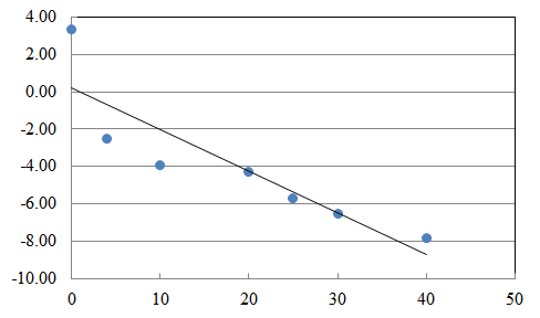
近似に使いたい関数
$y=ax^\frac{3}{2}+b$
- つまり,aとbのパラメータを決めたいということである。
コード
fitting.r
x1<-c(0,4,10,20,25,30,40)
y1<-c(3.37E+00,-2.48E+00,-3.92E+00,-4.30E+00,-5.72E+00,-6.54E+00,-7.83E+00)
fm<-nls(y1~a*x1^(3/2)+b,start=c(a=1,b=1),trace=TRUE)
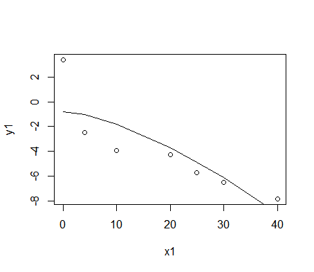
plot(x1,y1)
lines(x1,fitted(fm))
決定されたパラメータの値を見る
- summary関数を使う。
> summary(fm)

Formula: y ~ a * x^(3/2) + b

Parameters:
  Estimate Std. Error t value Pr(>|t|)
a -0.03254    0.01015  -3.204   0.0239 *
b -0.79665    1.30549  -0.610   0.5684
---
Signif. codes:  0 ‘***’ 0.001 ‘**’ 0.01 ‘*’ 0.05 ‘.’ 0.1 ‘ ’ 1

Residual standard error: 2.3 on 5 degrees of freedom

Number of iterations to convergence: 1
Achieved convergence tolerance: 1.527e-07
fitting curveの各点の値を取得する
data.frame(fitted(fm))
> data.frame(fitted(fm))
  fitted.fm.
1 -0.7966525
2 -1.0569395
3 -1.8255273
4 -3.7067501
5 -4.8636375
6 -6.1428431
7 -9.0276515
7つのデータは,x1のそれぞれの位置でのfitting curve上の値を出力している。
インプットテストデータとの相関係数を計算すると,0.82であった。
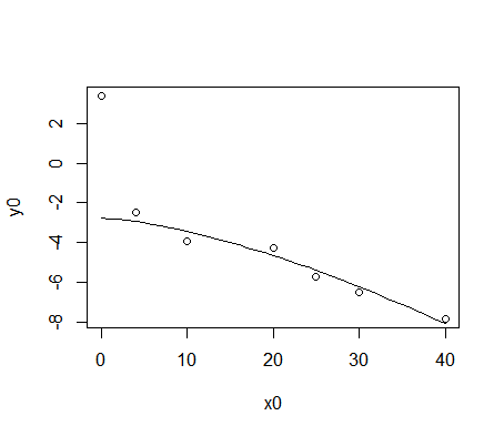
非線形近似曲線を滑らかにプロットする
方法は2つある。
(1) fitting curveの出力するデータポイントを細かく刻む。
(2) fitting curveのparameterから関数そのものをプロットする。
どちらも綺麗な曲線が描ける。
しかし,(1)の場合は predict 関数を用いるが,fittingに用いたinputデータの値の範囲内でしかプロットできない。
したがって,(2)の方が万能である。以下に例を示す。
fitting02.r
x0<-c(0,4,10,20,25,30,40)
y0<-c(3.37E+00,-2.48E+00,-3.92E+00,-4.30E+00,-5.72E+00,-6.54E+00,-7.83E+00)

x1<-c(4,10,20,25,30,40)
y1<-c(-2.48E+00,-3.92E+00,-4.30E+00,-5.72E+00,-6.54E+00,-7.83E+00)

fm1<-nls(y1~a*x1^(3/2)+b,start=c(a=1,b=1),trace=TRUE)

plot(x0,y0)
# lines(x1,fitted(fm1))


# For high resolution
## (1) Try1: generation of many points
## *** can plot only range of input data
# r <- range(x1)
# x2 <- seq(r[1],r[2],length.out=200)
# y2 <- predict(fm1,list(x1=x2))
# lines(x2,y2)

## (2) Try2
## *** just plot the function
a1 <- coef(fm1)[1]
b1 <- coef(fm1)[2]
lines(x<-c(0:40),a1*x^(3/2)+b1)
この例では,最初のデータはフィッティング解析から除外してある。
参考
- nls 関数の基本的な使い方
- 非線形近似曲線を滑らかにプロットする