KerasでIMDB映画レビューのデータセットを使って2クラス分類をしてみました。
IMDBデータセットは、各レビューに対して、肯定/否定(ネガポジ)のラベルづけがされているものになります。
IMDBデータセットのKerasの公式ドキュメントの説明は以下。
IMDB映画レビューデータセット
IMDBデータセットは、学習用に25000、テスト用に25000のそれぞれレビューデータがあるデータセットです。positive、negativeの割合は、学習用、テスト用ともに50%ずつ分けられています。
Kerasを使った浅いニューラルネットで分類してみました。
動作環境
- Mac Book Pro 10.13.2
- Python 3.5.2
- Tensorflow 1.5.0
- Keras 2.1.4
- Jupyter 1.0.0
実装
IMDBデータセットの読み込み
まずはIMDBデータセットをダウンロードしてきます。Kerasはデータセットのダウンロードをkeras.datasets.imdbで行えます。num_words=10000は、出現する頻度が上位10000の単語のみをデータとして使用することを指定する変数です。
学習用とテスト用のデータを読み込んだ後、train_dataの1番目のレビューデータを出力してみます。出力は整数のリストで、これは単語がそれぞれインデックスにエンコードされているためです。
from keras.datasets import imdb

(train_data, train_labels), (test_data, test_labels) = imdb.load_data(num_words=10000)

train_data[0]
[1, 14, 22, 16, 43, ... 5345, 19, 178, 32]
また、ラベルは以下のようになります。0がnegativeで、1がpositiveを示しています。
train_labels[0]
1
ちなみに、私のMacの環境下において、ダウンロードしてきたデータセットは以下に保存されていました。(80MBほど)
~/.keras/datasets/imdb.npz
整数のインデックスになっているデータをテキストデータに変換して確認してみます。
そのため、単語がkeyでインデックスがvalueとして辞書になっているjsonデータをダウンロードします。
word_index = imdb.get_word_index()
jsonは以下のような中身になっています。
{
  "fawn": 34701,
  "tsukino": 52006,
  "nunnery": 52007,
  "sonja": 16816,
  "vani": 63951,
  "woods": 1408,
  "spiders": 16115,
  "hanging": 2345,
       :
}
ダウンロードした辞書によって、整数のインデックスのリストで表されているデータを文字列にデコードします。
3を指定しているのは、0,1,2が学習には不要な文字のインデックスになっているためです。1番目のデータのテキストを表示してみます。
reverse_word_index = dict([(value, key) for (key, value) in word_index.items()])
decoded_review = ' '.join([reverse_word_index.get(i - 3, '?') for i in train_data[0]])

decoded_review
"? this film was just brilliant casting location scenery story direction everyone's really suited the part they played and you could just imagine being there robert ? is an amazing actor and now the same being director ? father came from the same scottish island as myself so i loved the fact there was a real connection with this film the witty remarks throughout the film were great it was just brilliant so much that i bought the film as soon as it was released for ? and would recommend it to everyone to watch and the fly fishing was amazing really cried at the end it was so sad and you know what they say if you cry at a film it must have been good and this definitely was also ? to the two little boy's that played the ? of norman and paul they were just brilliant children are often left out of the ? list i think because the stars that play them all grown up are such a big profile for the whole film but these children are amazing and should be praised for what they have done don't you think the whole story was so lovely because it was true and was someone's life after all that was shared with us all"
データの前処理
データは、整数のインデックスになっており、このままでは学習の入力に使えないので、One-hotベクトルに変換します。ここでは、One-hotベクトルの次元は10000とし、出現した単語に1を割り当てます。このOne-hotベクトルへの変換では、単語の出現頻度や並び順といった情報は落ちています。
import numpy as np

def vectorize_sequences(sequences, dimension=10000):
    results = np.zeros((len(sequences), dimension))
    for i, sequence in enumerate(sequences):
        results[i, sequence] = 1.
    return results

x_train = vectorize_sequences(train_data)
x_test = vectorize_sequences(test_data)

x_train[0]
array([0., 1., 1., ..., 0., 0., 0.])
またラベルも整数ではなく、浮動小数に変換します。
y_train = np.asarray(train_labels).astype('float32')
y_test = np.asarray(test_labels).astype('float32')

y_train
array([1., 0., 0., ..., 0., 1., 0.], dtype=float32)
これでニューラルネットに入力するための準備ができました。
ネットワークの構築
次に学習させるネットワークを定義します。layers.Denseを使用して、全結合層のみのネットワークとなります。ネットワークとしては、3層の浅いニューラルネットで、1,2番目の隠れ層のユニットは16、活性化関数はreluを使用します。また、input_shapeにOne-hotベクトルの次元を指定します。2クラス分類なので、最後の層の出力はsigmoid層で、どちらのクラスであるかの確率を出力します。
from keras import models
from keras import layers

model = models.Sequential()
model.add(layers.Dense(16, activation='relu', input_shape=(10000,)))
model.add(layers.Dense(16, activation='relu'))
model.add(layers.Dense(1, activation='sigmoid'))
モデル情報は以下のように出力できます。全パラメータ数は160,305のようです。
model.summary()
_________________________________________________________________
Layer (type)                 Output Shape              Param #
=================================================================
dense_1 (Dense)              (None, 16)                160016
_________________________________________________________________
dense_2 (Dense)              (None, 16)                272
_________________________________________________________________
dense_3 (Dense)              (None, 1)                 17
=================================================================
Total params: 160,305
Trainable params: 160,305
Non-trainable params: 0
_________________________________________________________________
学習設定
次に、学習の際のoptimizer、損失関数、metricsを指定します。optimizerにはrmsprop、損失関数においては今回は2クラス分類なのでbinary_crossentropyを指定しました。
model.compile(optimizer='rmsprop',
              loss='binary_crossentropy',
              metrics=['accuracy'])
また、学習データをtrain用と、validation用に分けます。今回はデータの前から10000個をvalidation用にしました。ここの分け方は、positiveとnegativeの数に不均衡が起きないようにランダムに分けたほうが精度がよくなるかも知れません。
x_val = x_train[:10000]
partial_x_train = x_train[10000:]
y_val = y_train[:10000]
partial_y_train = y_train[10000:]
学習結果
学習は以下のようにmodel.fitを実行して行います。epochsは20、バッチサイズは512に今回は設定しました。
history = model.fit(partial_x_train,
                    partial_y_train,
                    epochs=20,
                    batch_size=512,
                    validation_data=(x_val, y_val))
history_dict = history.history
model.fitはhistory objectを返します。history objectはメンバのhistoryを持っていて学習の際の情報を辞書として持っています。
history_dict.keys()
dict_keys(['val_loss', 'loss', 'acc', 'val_acc'])
以下のコードを実行して、lossの変化をグラフに表示してみます。
%matplotlib inline
import matplotlib.pyplot as plt

loss_values = history_dict['loss']
val_loss_values = history_dict['val_loss']
acc = history_dict['acc']

epochs = range(1, len(acc) + 1)

plt.plot(epochs, loss_values, 'bo', label='Training loss')
plt.plot(epochs, val_loss_values, 'b', label='Validation loss')
plt.title('Training and validation loss')
plt.xlabel('Epochs')
plt.ylabel('Loss')
plt.legend()

plt.show()
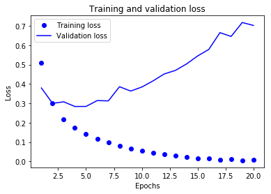
lossの変化は以下となりました。training lossは0近くになっていますが、validation lossがおよそ5epochで最小になってから、上がり続けており、過学習の状態です。
精度についても以下のコードを実行して確認してみます。
val_acc_values = history_dict['val_acc']

plt.plot(epochs, acc, 'bo', label='Training acc')
plt.plot(epochs, val_acc_values, 'b', label='Validation acc')
plt.title('Training and validation accuracy')
plt.xlabel('Epochs')
plt.ylabel('Accuracy')
plt.legend()

plt.show()
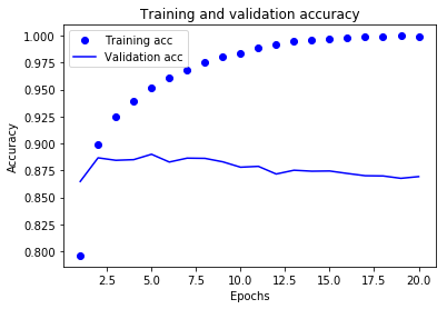
精度がtrainでは、1に近くなっているのに対し、validationでは0.88ほどで差があり過学習を示しています。過学習を改善するため、データの分け方、隠れ層のユニット数や層の数を調整する必要がありそうです。
ちなみに、train,validationの両方のデータを合わせて学習した時のtestに対する精度を出してみました。
model = models.Sequential()
model.add(layers.Dense(16, activation='relu', input_shape=(10000,)))
model.add(layers.Dense(16, activation='relu'))
model.add(layers.Dense(1, activation='sigmoid'))

model.compile(optimizer='rmsprop',
              loss='binary_crossentropy',
              metrics=['accuracy'])

model.fit(x_train, y_train, epochs=4, batch_size=512)
results = model.evaluate(x_test, y_test)
results
[0.32485373953819274, 0.87288]
testデータに対する精度は87%ほどになりました。精度を改善するためにユニット数や層数を変えたり、dropoutなどを試して検証しても良さそうですね。
ソースコードまとめ
全体のコードになります。
%matplotlib inline
import matplotlib.pyplot as plt
import numpy as np

from keras import models
from keras import layers
from keras.datasets import imdb

(train_data, train_labels), (test_data, test_labels) = imdb.load_data(num_words=10000)

word_index = imdb.get_word_index()
reverse_word_index = dict([(value, key) for (key, value) in word_index.items()])
decoded_review = ' '.join([reverse_word_index.get(i - 3, '?') for i in train_data[0]])

print(decoded_review)

def vectorize_sequences(sequences, dimension=10000):
    results = np.zeros((len(sequences), dimension))
    for i, sequence in enumerate(sequences):
        results[i, sequence] = 1.
    return results

x_train = vectorize_sequences(train_data)
x_test = vectorize_sequences(test_data)

y_train = np.asarray(train_labels).astype('float32')
y_test = np.asarray(test_labels).astype('float32')

model = models.Sequential()
model.add(layers.Dense(16, activation='relu', input_shape=(10000,)))
model.add(layers.Dense(16, activation='relu'))
model.add(layers.Dense(1, activation='sigmoid'))

model.summary()

model.compile(optimizer='rmsprop',
              loss='binary_crossentropy',
              metrics=['accuracy'])

x_val = x_train[:10000]
partial_x_train = x_train[10000:]
y_val = y_train[:10000]
partial_y_train = y_train[10000:]

history = model.fit(partial_x_train,
                    partial_y_train,
                    epochs=20,
                    batch_size=512,
                    validation_data=(x_val, y_val))

history_dict = history.history
print(history_dict.keys())

loss_values = history_dict['loss']
val_loss_values = history_dict['val_loss']
acc = history_dict['acc']

epochs = range(1, len(acc) + 1)

plt.plot(epochs, loss_values, 'bo', label='Training loss')
plt.plot(epochs, val_loss_values, 'b', label='Validation loss')
plt.title('Training and validation loss')
plt.xlabel('Epochs')
plt.ylabel('Loss')
plt.legend()

plt.show()

val_acc_values = history_dict['val_acc']

plt.plot(epochs, acc, 'bo', label='Training acc')
plt.plot(epochs, val_acc_values, 'b', label='Validation acc')
plt.title('Training and validation accuracy')
plt.xlabel('Epochs')
plt.ylabel('Accuracy')
plt.legend()

plt.show()

model = models.Sequential()
model.add(layers.Dense(16, activation='relu', input_shape=(10000,)))
model.add(layers.Dense(16, activation='relu'))
model.add(layers.Dense(1, activation='sigmoid'))

model.compile(optimizer='rmsprop',
              loss='binary_crossentropy',
              metrics=['accuracy'])

model.fit(x_train, y_train, epochs=4, batch_size=512)
results = model.evaluate(x_test, y_test)
print(results)