最近、Meta-Learningについて勉強したのでMeta-Learningの1つの手法であるMetric Learningについて記事をかいてみました。Metric Learningの基本的な手法であるSiamese NetworkをKerasとPytorchで実装して簡単な精度評価まで行いました。
Kerasの実装はシンプルなSiamese Networkを実装したもので、Pytorchの実装は以下の論文のアーキテクチャを実装し、論文と同様に精度評価してみたものになります。
Siamese Neural Networks for One-shot Image Recognition
Meta-Learningとは?
Meta-Learning: Learning to Learn Fast より引用
Meta-learning, also known as “learning to learn”, intends to design models that can learn new skills or adapt to new environments rapidly with a few training examples. There are three common approaches: 1) learn an efficient distance metric (metric-based); 2) use (recurrent) network with external or internal memory (model-based); 3) optimize the model parameters explicitly for fast learning (optimization-based).
Meta-Learningは"learning to learn"という言葉で表されるように学習の仕方を学習するといったような技術になります。Meta-Learningにより、少数の学習データから新しいスキルを学習したり、新しい環境に適応することができます。
Meta-Learningには以下の3つの一般的なアプローチがあります。
- Metric-Based
- Convolutional Siamese Neural Network
- Matching Networks
- Relation Network
- Prototypical Networks
- Model-Based
- Memory-Augmented Neural Networks
- Meta Networks
- Optimization-Based
- LSTM Meta-Learner
- MAML
- Reptile
今回は、この中で Metric-Basedな手法であるSiamese Neural NetworkをKerasとPytorchで実装してみました。
Metric Learningとは?
Qiita: Siamese Neural Networks for One-shot Image Recognition より引用
Metric Learningとはデータ間の計量(類似度や距離など)を学習する手法です。計量を学習するということは、「特徴空間を学習する」,「埋め込み方を学習する」と捉えることもできます。僕的には埋め込み方を学習するという考え方が一番しっくりきています。直感的なイメージとしては、意味の近いデータは近く、意味の遠いデータは遠くなるように特徴空間を学習してる感じです。
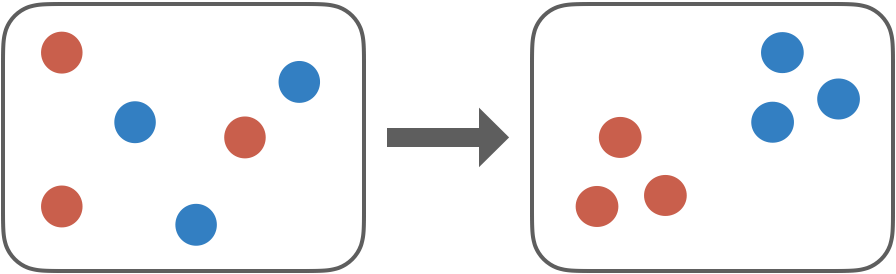
Metric Learningは意味的に近いデータが類似度や距離などで近くなるように学習し、意味的に離れているものは遠くなるように学習し、データに対し有用な特徴量を得ることができます。例えば、同じ犬の画像データは近くなるように埋め込みの特徴量を学習し、犬と猫の画像データは互いに遠くなるように学習します。
また、Metric Learningはデータのクラスラベルを直接予測するわけではなく、距離的な意味表現を学習するため、one-shot learningやfew-shot learningといった少数データからクラス分類を行うタスクに適用することが可能です。
Metric Learning(Siamese Network)の学習
Siamese Neural Networks for One-shot Image Recognition 論文のSiamese Networkでは以下のような入出力のタスク(Verification task)をといてモデル学習をしています。
- 入力: 2つのデータを組みにしたもの
- 出力: 2つのデータが意味的に近いかのスコア(0~1)
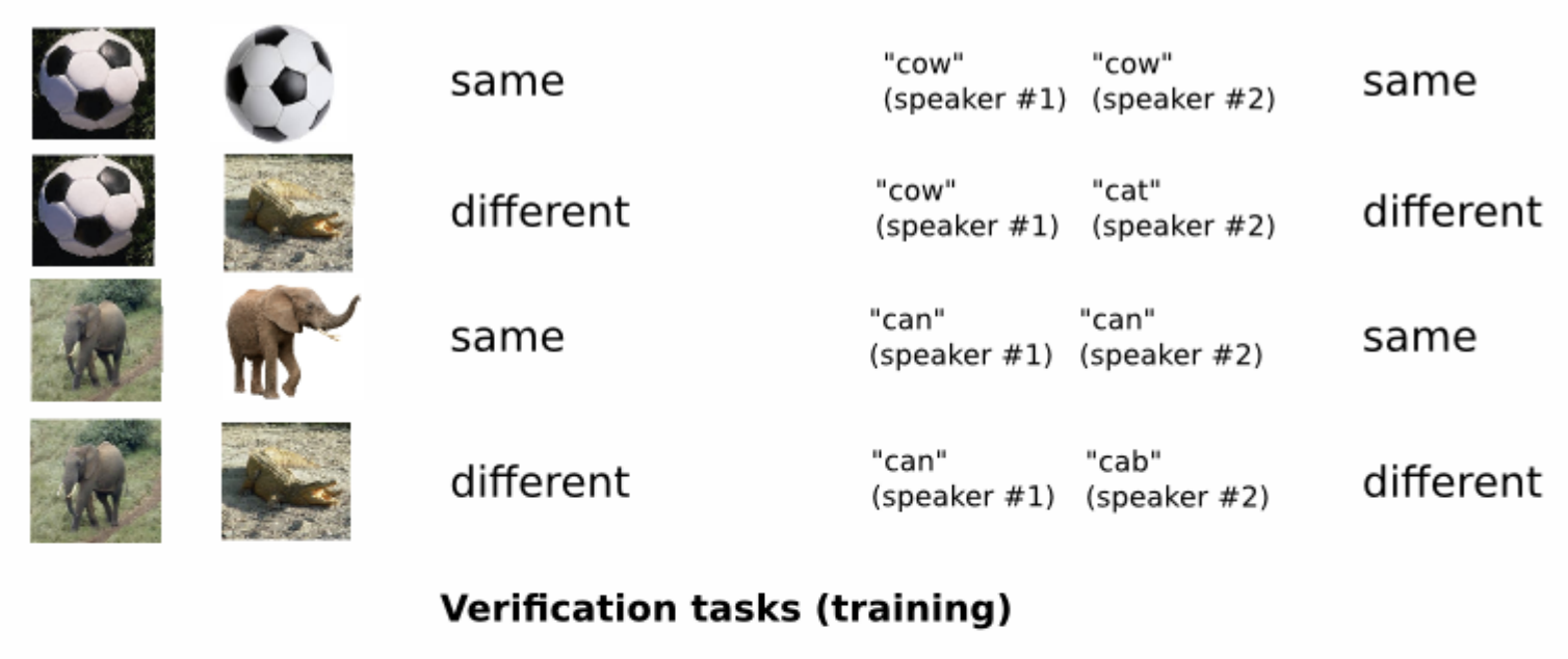
上の図の例から、deep learningによってサッカーボールどうしは近い特徴空間に埋め込むように学習し、サッカーボールとワニの組み合わせは特徴空間で遠くなるように学習します。
One-shot Learning

論文では、Verification tasksの精度評価と別にone-shot learningでの精度評価もしています。
テスト画像$x$と学習データにはなかった各クラスを代表する画像の集合$\{x_c\}_{c=1}^C$(各クラス1つのデータ)が与えられているとすると以下の式に相当する最大の類似度を持ったクラス$c$を予測結果とすればone-shot learningが可能です。
$$
C^*=argmax_c p^{(c)}
$$
Siamese Networkのアーキテクチャ
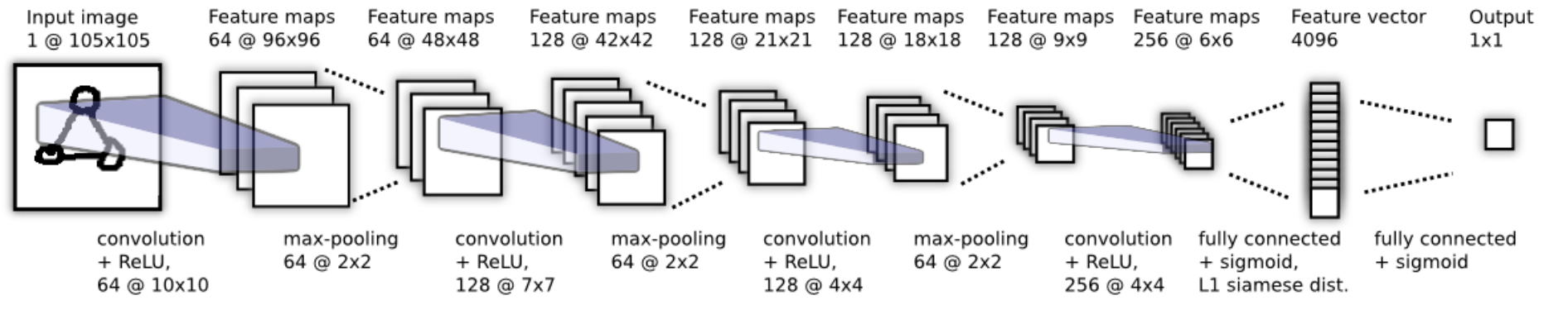
Siamese Networkはネットワークのパラメータが共有されており、2つのデータは同じ重みを持ったネットワークに入力されます。Outputの1x1の出力で1(同じ人の顔の組み) or 0(異なる人の顔の組み)を予測するように学習します。
one-shot learningの場合には、各クラスを代表する画像の集合$\{x_c\}_{c=1}^C$(各クラス1つのデータ)のそれぞれをモデルに入力し、得られたFeature vector(4096次元)を検索できるように保存しておきます。そして、テスト画像$x$を別途入力し、得られたFeature vectorと保存されているFeature vectorの類似度(距離)をそれぞれ計算し、最大の類似度のデータと同じクラスを返します。
実装
Keras, Pytorch実装のレポジトリは以下にありますので、動かしてみたい方、詳細な実装を知りたい方は参照していただければと思います。(Verification taskの精度評価しかまだできていないですが。。。)
Pytorch実装は以下のレポジトリのコードを参考に実装しています。
https://github.com/matbambbang/siamese-networks-omniglot-pytorch
Keras実装
AT&T Database of Faces dataset(学習データセット)
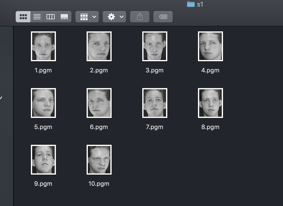
Keras実装では顔認証用のデータセットであるAT&T Database of Faces datasetを使用して学習します。
データセットの内容としてはs1~s40まで40人の人の顔画像があり、1人あたり10枚の画像があるデータセットになっています。s1フォルダを見ると以下のようになっています。Deep Learningを学習するには1クラスあたりの学習データが非常に少ないデータであると思います。
詳細な実装
Siamese Network特有と思われる箇所だけ簡単に説明させていただきます。
x_genuine_pairに2枚の同じ人の顔の画像を組みして学習データとして作成します。
np.random.randint(10)で10枚ある画像の2枚をランダムに選び、重複しないようにして組みにします。同じ人の顔画像の組みの場合、ラベルは1、異なる人同士の組みの場合は0になります。
x_genuine_pairとx_imposite_pairのデータ数は、データ不均衡にならないように同じ数だけ作成するように処理しています。
def get_data(seize, total_sample_size):
    # read the image
    image = read_image('data/orl_faces/s' + str(1) + '/' + str(1) + '.pgm', 'rw+')
    # reduce the size
    image = image[::size, ::size]
    # get the new size
    dim1 = image.shape[0]
    dim2 = image.shape[1]

    count = 0

    # initialize the numpy array with the shape of [total_sample, no_of_pairs, dim1, dim2]
    x_genuine_pair = np.zeros([total_sample_size, 2, 1, dim1, dim2])  # 2 is for pairs
    y_genuine = np.zeros([total_sample_size, 1])

    for i in range(40):
        for j in range(int(total_sample_size/40)):
            ind1 = 0
            ind2 = 0

            # read images from same directory (genuine pair)
            while ind1 == ind2:
                ind1 = np.random.randint(10)
                ind2 = np.random.randint(10)

            # read the two images
            img1 = read_image('data/orl_faces/s' + str(i+1) + '/' + str(ind1 + 1) + '.pgm', 'rw+')
            img2 = read_image('data/orl_faces/s' + str(i+1) + '/' + str(ind2 + 1) + '.pgm', 'rw+')

            # reduce the size
            img1 = img1[::size, ::size]
            img2 = img2[::size, ::size]

            # store the images to the initialized numpy array
            x_genuine_pair[count, 0, 0, :, :] = img1
            x_genuine_pair[count, 1, 0, :, :] = img2

            # as we are drawing images from the same directory we assign label as 1. (genuine pair)
            y_genuine[count] = 1
            count += 1

    count = 0
    x_imposite_pair = np.zeros([total_sample_size, 2, 1, dim1, dim2])
    y_imposite = np.zeros([total_sample_size, 1])

    for i in range(int(total_sample_size/10)):
        for j in range(10):
            # read images from different direcoty (imposite pair)
            while True:
                ind1 = np.random.randint(40)
                ind2 = np.random.randint(40)
                if ind1 != ind2:
                    break

            img1 = read_image('data/orl_faces/s' + str(ind1 + 1) + '/' + str(j + 1) + '.pgm', 'rw+')
            img2 = read_image('data/orl_faces/s' + str(ind2 + 1) + '/' + str(j + 1) + '.pgm', 'rw+')

            img1 = img1[::size, ::size]
            img2 = img2[::size, ::size]

            x_imposite_pair[count, 0, 0, :, :] = img1
            x_imposite_pair[count, 1, 0, :, :] = img2

            # as we are drawing images from the different directory we assign label as 0. (imposite pair)
            y_imposite[count] = 0
            count += 1

    # now, concatenate, genuine pairs and imposite pair to get the whole data
    X = np.concatenate([x_genuine_pair, x_imposite_pair], axis=0) / 255
    Y = np.concatenate([y_genuine, y_imposite], axis=0)

    return X, Y
Keras実装のニューラルネットのアーキテクチャは論文と同じではなく、シンプルなアーキテクチャで実装しています。
def build_base_network(input_shape, nb_filter=[6, 12], kernel_size=3):
    seq = Sequential()

    # convolutional layer 1
    seq.add(Conv2D(nb_filter[0], (kernel_size, kernel_size), input_shape=input_shape,
                   padding='valid', data_format="channels_first"))
    seq.add(Activation('relu'))
    seq.add(MaxPool2D(pool_size=(2, 2)))
    seq.add(Dropout(.25))

    # convolutional layer 2
    seq.add(Conv2D(nb_filter[1], (kernel_size, kernel_size),
                   padding='valid', data_format="channels_first"))
    seq.add(Activation('relu'))
    seq.add(MaxPool2D(pool_size=(2, 2), data_format="channels_first"))
    seq.add(Dropout(0.25))

    # flatten
    seq.add(Flatten())
    seq.add(Dense(128, activation='relu'))
    seq.add(Dropout(0.1))
    seq.add(Dense(50, activation='relu'))
    return seq
データ間の類似度を計る関数としては今回ユークリッド距離を使っています。ここはcosine similarityなど色々選択肢があるかと思います。
def euclidean_distance(vects):
    x, y = vects
    return K.sqrt(K.sum(K.square(x - y), axis=1, keepdims=True))


def eucl_dist_output_shape(shapes):
    shape1, shape2 = shapes
    return (shape1[0], 1)


def contrastive_loss(y_true, y_pred):
    margin = 1
    return K.mean(y_true * K.square(y_pred) + (1 - y_true) * K.square(K.maximum(margin - y_pred, 0)))
2つの画像の入力に対しニューラルネットのモデルはパラメータを共有しています。入力をそれぞれ定義し、モデルに渡している箇所に注意していただければと思います。
# load dataset
    X, Y = get_data(size, total_sample_size)
    print(X.shape)
    print(Y.shape)

    x_train, x_test, y_train, y_test = train_test_split(X, Y, test_size=0.25)

    input_dim = x_train.shape[2:]
    img_a = Input(shape=input_dim)
    img_b = Input(shape=input_dim)

    base_network = build_base_network(input_dim)
    feat_vecs_a = base_network(img_a)
    feat_vecs_b = base_network(img_b)

    distance = Lambda(euclidean_distance, output_shape=eucl_dist_output_shape)([feat_vecs_a, feat_vecs_b])

    epochs = 20
    rms = RMSprop()

    model = Model(input=[img_a, img_b], output=distance)
    model.compile(loss=contrastive_loss, optimizer=rms)
学習方法
cd face
データセットを次のサイトからダウンロード https://www.kaggle.com/kasikrit/att-database-of-faces
unzip att-database-of-faces.zip
python main.py
Train on 11250 samples, validate on 3750 samples
Epoch 1/20
 - 2s - loss: 0.2272 - val_loss: 0.3171
Epoch 2/20
 - 1s - loss: 0.1513 - val_loss: 0.2144
Epoch 3/20
 - 1s - loss: 0.1198 - val_loss: 0.1509
Epoch 4/20
 - 1s - loss: 0.0998 - val_loss: 0.1356
Epoch 5/20
 - 1s - loss: 0.0850 - val_loss: 0.1435
Epoch 6/20
 - 1s - loss: 0.0750 - val_loss: 0.1262
Epoch 7/20
 - 1s - loss: 0.0665 - val_loss: 0.0892
Epoch 8/20
 - 1s - loss: 0.0605 - val_loss: 0.0574
Epoch 9/20
 - 1s - loss: 0.0555 - val_loss: 0.0676
Epoch 10/20
 - 1s - loss: 0.0519 - val_loss: 0.0443
Epoch 11/20
 - 1s - loss: 0.0480 - val_loss: 0.0658
Epoch 12/20
 - 1s - loss: 0.0443 - val_loss: 0.0531
Epoch 13/20
 - 1s - loss: 0.0415 - val_loss: 0.0553
Epoch 14/20
 - 1s - loss: 0.0388 - val_loss: 0.0448
Epoch 15/20
 - 1s - loss: 0.0377 - val_loss: 0.0489
Epoch 16/20
 - 1s - loss: 0.0358 - val_loss: 0.0448
Epoch 17/20
 - 1s - loss: 0.0336 - val_loss: 0.0344
Epoch 18/20
 - 1s - loss: 0.0309 - val_loss: 0.0381
Epoch 19/20
 - 1s - loss: 0.0299 - val_loss: 0.0305
Epoch 20/20
 - 1s - loss: 0.0285 - val_loss: 0.0303
0.9492424242424242
Pytorch実装
Pytorch実装は以下の場所にありますので、詳細が気になる方はご参照ください。
https://github.com/kambehmw/siamese-networks/tree/master/omniglot
Omniglot dataset(学習データセット)
Pytorch実装では、Siamese Neural Networks for One-shot Image Recognition 論文と同じOmniglot datasetで学習を行います。データセットとしては以下のように色々な言語の文字が集められたデータセットになります。
Omniglot dataset
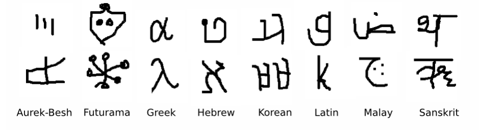
The Omniglot data set contains 50 alphabets. We split these into a background set of 30 alphabets and an evaluation set of 20 alphabets.
全体で50言語あり、そのうち30がbackgroundでtrain用、残りの20がevaluation用に分割されています。
学習方法
データセットダウンロードします。omniglot/data/に展開されるようになっています。
bash download_dataset.sh
以下で学習を実行。論文と同様にtraining exampleを30000作成して学習します。(no distortions)
精度評価は、学習に使っていないevaluation用データセット(全て学習に存在しないクラス)から2枚の画像の組みを400作成して、評価。
python main.py
Epoch 1
/home/kanbe.hiroyuki@wing.sysrdc.com/miniconda3/envs/py37-hands-on-meta-learning/lib/python3.7/site-packages/torch/nn/_reduction.py:43: UserWarning: size_average and reduce args will be deprecated, please use reduction='none' instead.
  warnings.warn(warning.format(ret))
Train mean loss (train): 0.64155
Verification loss : 0.58077
Verification accuracy : 0.728
Epoch 2
Train mean loss (train): 0.56825
Verification loss : 0.56835
Verification accuracy : 0.720
Epoch 3
Train mean loss (train): 0.43263
Verification loss : 0.46790
Verification accuracy : 0.787
Epoch 4
Train mean loss (train): 0.31896
Verification loss : 0.34038
Verification accuracy : 0.870
Epoch 5
Train mean loss (train): 0.21850
Verification loss : 0.30176
Verification accuracy : 0.868
Epoch 6
Train mean loss (train): 0.12765
Verification loss : 0.27595
Verification accuracy : 0.877
Epoch 7
Train mean loss (train): 0.05723
Verification loss : 0.27553
Verification accuracy : 0.892
Epoch 8
Train mean loss (train): 0.02791
Verification loss : 0.32576
Verification accuracy : 0.868
Epoch 9
Train mean loss (train): 0.01102
Verification loss : 0.34327
Verification accuracy : 0.892
Epoch 10
Train mean loss (train): 0.00365
Verification loss : 0.35693
Verification accuracy : 0.910
Epoch 11
Train mean loss (train): 0.00148
Verification loss : 0.33043
Verification accuracy : 0.912
   :
   :
Verification accuracyが0.9ほどで、以下の論文の画像の30k training no distortionsの90.61とほぼ同等の精度が出ています。

感想
- one-shot learningについて論文と同じ精度評価ができていないので、できればやりたい…
- Metric Learning手法を自然言語処理データにも適用してみたい