Plotlyを使う人にも家族がいることを、私たちは忘れていません。

はじめに

スーパーでブロッコリーを見るとPlotlyを連想する病気にかかっています。
自分の作業用によく使うPlotlyの使い方をまとめたので公開します。
実際にグリグリ動かしたい方はkaggleのkernelにアップしてるのでそちらでグリグリしてください。
https://www.kaggle.com/kageyama/how-to-use-plotly

※ちなみにPlotlyの3Dグラフをグリグリしたことがない人は、是非とも一度グリグリした方がいい。感動する。

データロード

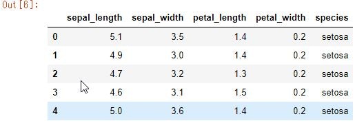
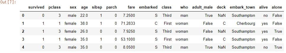
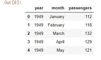
データはseabornから
iris,titanic,flightsの3つを適宜使用する。

import numpy as np
import pandas as pd

import plotly as py
from plotly.offline import init_notebook_mode, iplot
init_notebook_mode(connected=True)
import plotly.graph_objs as go
import plotly.figure_factory as ff
import seaborn as sns

iris_data = sns.load_dataset("iris")
titanic_data = sns.load_dataset('titanic')
flights_data = sns.load_dataset('flights')

iris_data.head()

titanic_data.head()

flights_data.head()

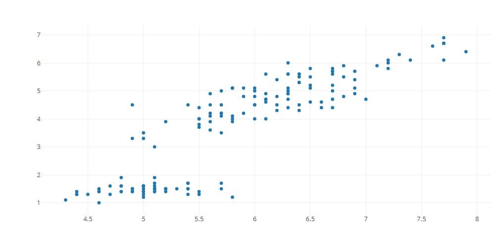
Scatter Plot

# Create a trace
trace = go.Scatter(
    x = iris_data['sepal_length'] ,
    y = iris_data['petal_length'] ,
    mode = 'markers'
)

tmp = [trace]

# Plot and embed in ipython notebook!
py.offline.iplot(tmp)

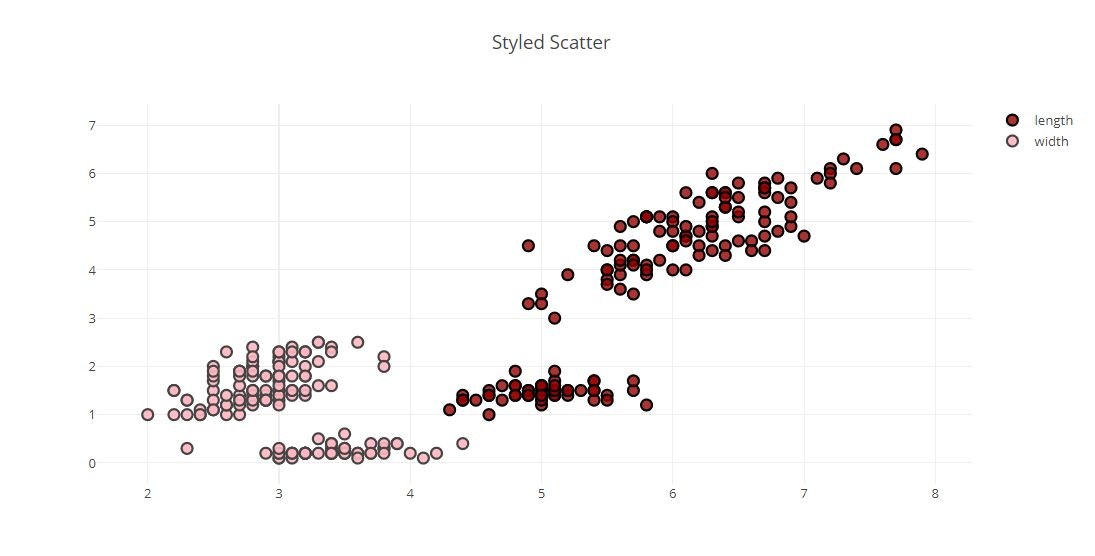
# Style Scatter Plots
trace0 = go.Scatter(
    x = iris_data['sepal_length'],
    y = iris_data['petal_length'],
    name = 'length',
    mode = 'markers',
    marker = dict(
        size = 10,
        color = 'rgba(152, 0, 0, .8)',
        line = dict(
            width = 2,
            color = 'rgb(0, 0, 0)'
        )
    )
)

trace1 = go.Scatter(
    x = iris_data['sepal_width'],
    y = iris_data['petal_width'],
    name = 'width',
    mode = 'markers',
    marker = dict(
        size = 10,
        color = 'rgba(255, 182, 193, .9)',
        line = dict(
            width = 2,
        )
    )
)

tmp = [trace0, trace1]

layout = dict(title = 'Styled Scatter',
              yaxis = dict(zeroline = False),
              xaxis = dict(zeroline = False)
             )

fig = dict(data=tmp, layout=layout)
py.offline.iplot(fig)

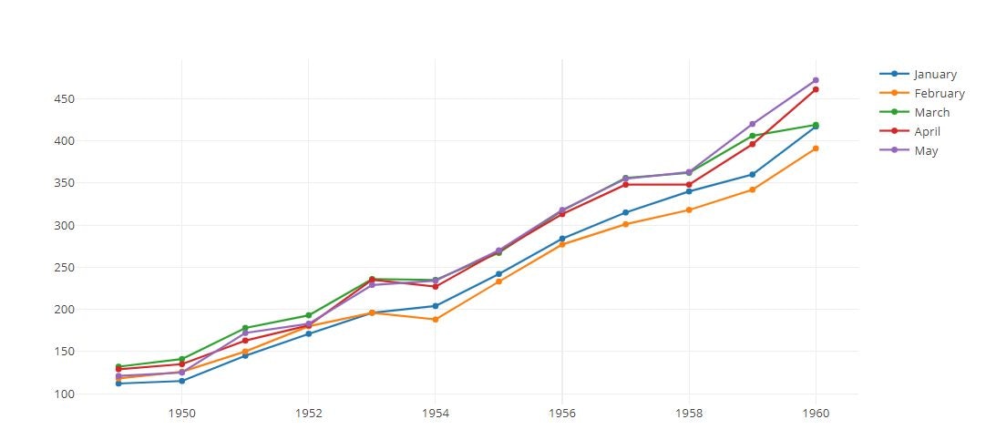
Line Plot

# Simple Line Plot

# Create a trace
trace1 = go.Scatter(
    x = flights_data[flights_data['month'] == 'January']['year'],
    y = flights_data[flights_data['month'] == 'January']['passengers'],
    name='January'
)

trace2 = go.Scatter(
    x = flights_data[flights_data['month'] == 'February']['year'],
    y = flights_data[flights_data['month'] == 'February']['passengers'],
    name='February'
)

trace3 = go.Scatter(
    x = flights_data[flights_data['month'] == 'March']['year'],
    y = flights_data[flights_data['month'] == 'March']['passengers'],
    name='March'
)

trace4 = go.Scatter(
    x = flights_data[flights_data['month'] == 'April']['year'],
    y = flights_data[flights_data['month'] == 'April']['passengers'],
    name='April'
)

trace5 = go.Scatter(
    x = flights_data[flights_data['month'] == 'May']['year'],
    y = flights_data[flights_data['month'] == 'May']['passengers'],
    name='May'
)

tmp = [trace1,trace2,trace3,trace4,trace5]

py.offline.iplot(tmp)

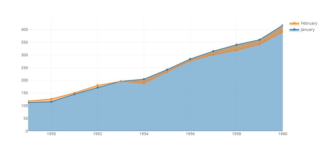
Filled Area Plot

trace1 = go.Scatter(
    x = flights_data[flights_data['month'] == 'January']['year'],
    y = flights_data[flights_data['month'] == 'January']['passengers'],
    name='January',
    fill='tozeroy'
)

trace2 = go.Scatter(
    x = flights_data[flights_data['month'] == 'February']['year'],
    y = flights_data[flights_data['month'] == 'February']['passengers'],
    name='February',
    fill='tonexty'
)


tmp = [trace1,trace2]

py.offline.iplot(tmp)

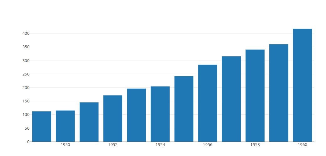
Bar Chart

# Basic
tmp = [go.Bar(
            x=flights_data[flights_data['month'] == 'January']['year'],
            y=flights_data[flights_data['month'] == 'January']['passengers'],
            name='January'
    )]
py.offline.iplot(tmp)

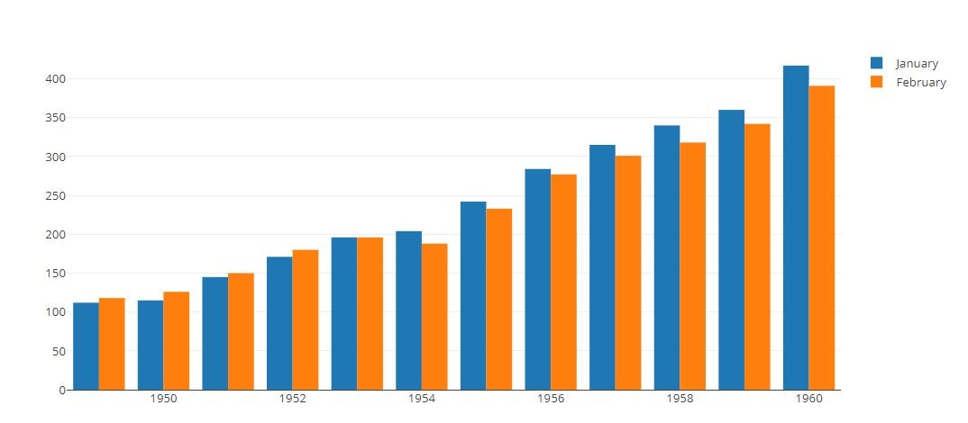
# Grouped Bar Chart
trace1 = go.Bar(
    x=flights_data[flights_data['month'] == 'January']['year'],
    y=flights_data[flights_data['month'] == 'January']['passengers'],
    name='January'
)
trace2 = go.Bar(
    x=flights_data[flights_data['month'] == 'February']['year'],
    y=flights_data[flights_data['month'] == 'February']['passengers'],
    name='February'
)

tmp = [trace1, trace2]
layout = go.Layout(
    barmode='group'
)

fig = go.Figure(data=tmp, layout=layout)
py.offline.iplot(fig)

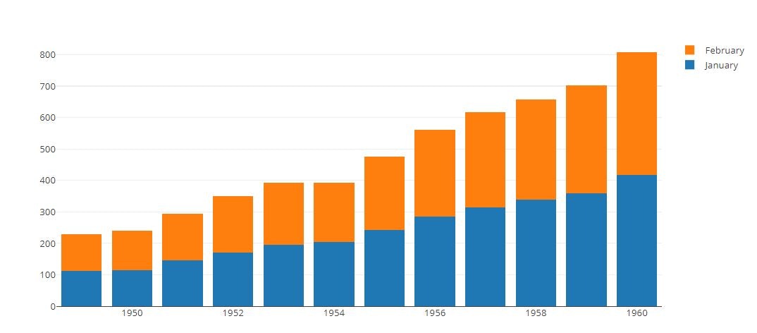
# Stacked Bar Chart
trace1 = go.Bar(
    x=flights_data[flights_data['month'] == 'January']['year'],
    y=flights_data[flights_data['month'] == 'January']['passengers'],
    name='January'
)
trace2 = go.Bar(
    x=flights_data[flights_data['month'] == 'February']['year'],
    y=flights_data[flights_data['month'] == 'February']['passengers'],
    name='February'
)

tmp = [trace1, trace2]
layout = go.Layout(
    barmode='stack'
)

fig = go.Figure(data=tmp, layout=layout)
py.offline.iplot(fig)

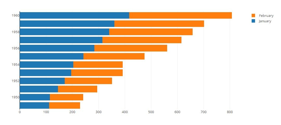
# Horizontal Bar Chart
trace1 = go.Bar(
    y=flights_data[flights_data['month'] == 'January']['year'],
    x=flights_data[flights_data['month'] == 'January']['passengers'],
    name='January',
    orientation = 'h',
)
trace2 = go.Bar(
    y=flights_data[flights_data['month'] == 'February']['year'],
    x=flights_data[flights_data['month'] == 'February']['passengers'],
    name='February',
    orientation = 'h',
)

tmp = [trace1, trace2]
layout = go.Layout(
    barmode='stack'
)

fig = go.Figure(data=tmp, layout=layout)
py.offline.iplot(fig)

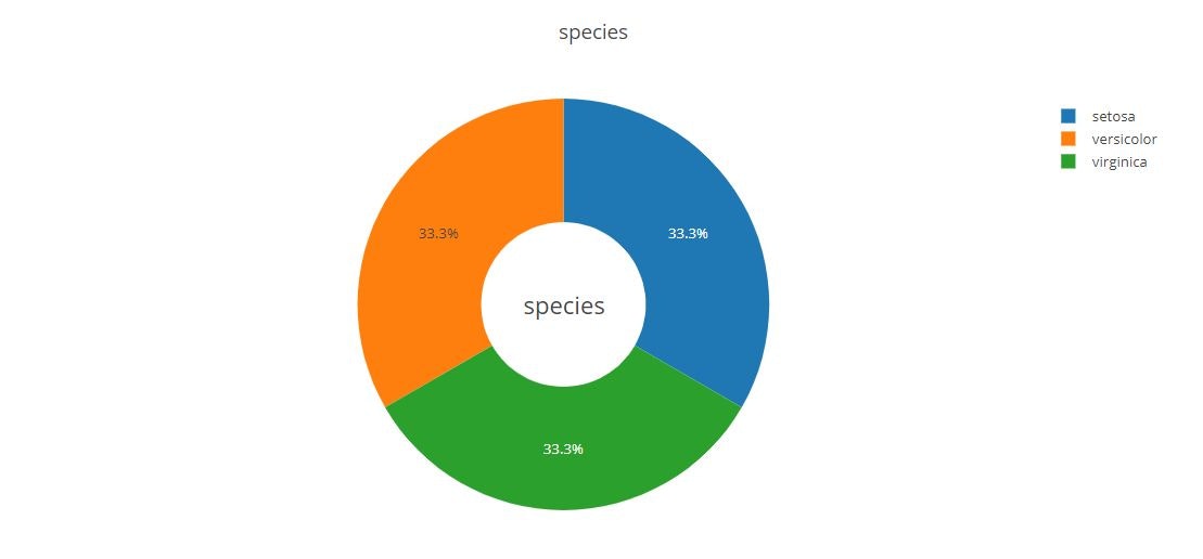
Pie Chart

# Basic
labels=['setosa','versicolor','virginica']
values=[len(iris_data[iris_data['species']=='setosa']),
        len(iris_data[iris_data['species']=='versicolor']),
        len(iris_data[iris_data['species']=='virginica'])]

trace=go.Pie(labels=labels, values=values)

py.offline.iplot([trace])

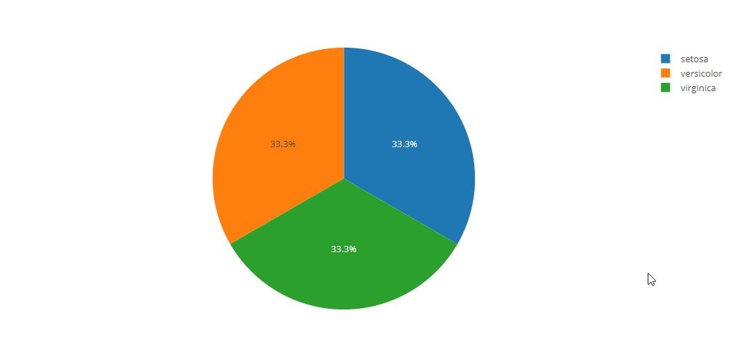
fig = {
  "data": [
    {
      "values": [len(iris_data[iris_data['species']=='setosa']),
        len(iris_data[iris_data['species']=='versicolor']),
        len(iris_data[iris_data['species']=='virginica'])],
      "labels": ['setosa','versicolor','virginica'],
      "domain": {"column": 0},
      "name": "species",
      "hoverinfo":"label+percent+name",
      "hole": .4,
      "type": "pie"
    }],
  "layout": {
        "title":"species",
        "grid": {"rows": 1, "columns": 1},
        "annotations": [
            {
                "font": {
                    "size": 20
                },
                "showarrow": False,
                "text": "species",
                "x": 0.5,
                "y": 0.5
            }
        ]
    }
}
py.offline.iplot(fig)

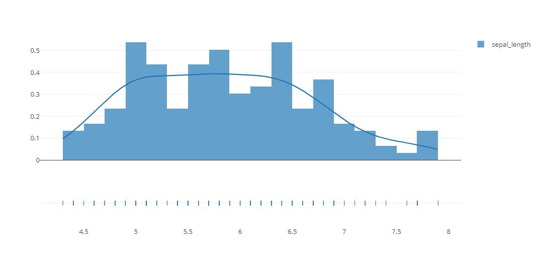
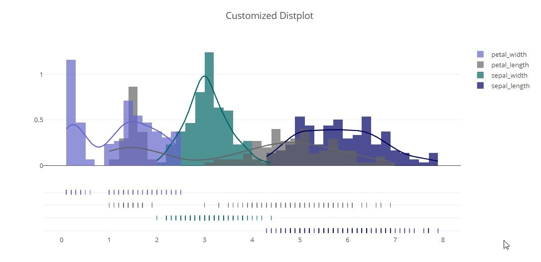
Distplot

x = iris_data['sepal_length'] 
hist_data = [x]
group_labels = ['sepal_length']

fig = ff.create_distplot(hist_data, group_labels,bin_size=.2)
py.offline.iplot(fig)

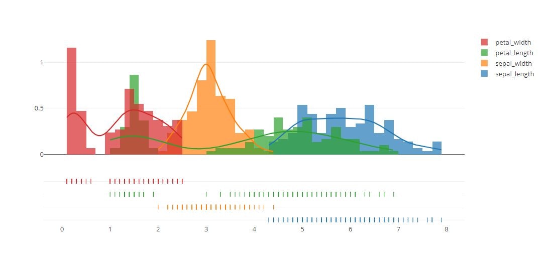
# Add histogram data
x1 = iris_data['sepal_length'] 
x2 = iris_data['sepal_width']  
x3 = iris_data['petal_length'] 
x4 = iris_data['petal_width'] 

# Group data together
hist_data = [x1, x2, x3, x4]

group_labels = ['sepal_length', 'sepal_width', 'petal_length', 'petal_width']

# Create distplot with custom bin_size
fig = ff.create_distplot(hist_data, group_labels, bin_size=.2)

# Plot!
py.offline.iplot(fig)

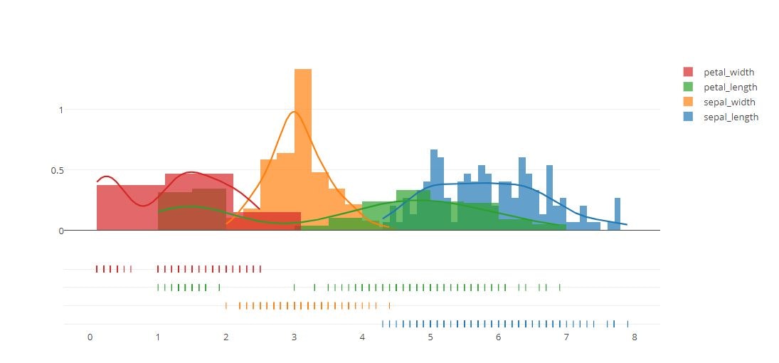
# Create distplot with custom bin_size
fig = ff.create_distplot(hist_data, group_labels, bin_size=[.1, .25, .5, 1])

# Plot!
py.offline.iplot(fig)

rug_text_one = ['a', 'b', 'c', 'd', 'e',
                'f', 'g', 'h', 'i', 'j', 
                'k', 'l', 'm', 'n', 'o',
                'p', 'q', 'r', 's', 't', 
                'u', 'v', 'w', 'x', 'y', 'z'] 

rug_text_two = ['aa', 'bb', 'cc', 'dd', 'ee',
                'ff', 'gg', 'hh', 'ii', 'jj', 
                'kk', 'll', 'mm', 'nn', 'oo',
                'pp', 'qq', 'rr', 'ss', 'tt', 
                'uu', 'vv', 'ww', 'xx', 'yy', 'zz'] 

rug_text_three = ['aaa', 'bbb', 'ccc', 'ddd', 'eee',
                'fff', 'ggg', 'hhh', 'iii', 'jjj', 
                'kkk', 'lll', 'mmm', 'nnn', 'ooo',
                'ppp', 'qqq', 'rrr', 'sss', 'ttt', 
                'uuu', 'vvv', 'www', 'xxx', 'yyy', 'zzz'] 

rug_text_four = ['aaaa', 'bbbb', 'cccc', 'dddd', 'eeee',
                'ffff', 'gggg', 'hhhh', 'iiii', 'jjjj', 
                'kkkk', 'llll', 'mmmm', 'nnnn', 'oooo',
                'pppp', 'qqqq', 'rrrr', 'ssss', 'tttt', 
                'uuuu', 'vvvv', 'wwww', 'xxxx', 'yyyy', 'zzzz'] 

rug_text = [rug_text_one, rug_text_two,rug_text_three,rug_text_four]

colors = ['rgb(0, 0, 100)', 'rgb(0, 100, 100)','rgb(100, 100, 100)','rgb(100, 100, 200)']

fig = ff.create_distplot(
    hist_data, group_labels, bin_size=.2,
    rug_text=rug_text, colors=colors)

fig['layout'].update(title='Customized Distplot')

# Plot!
py.offline.iplot(fig)

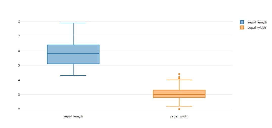
trace0 = go.Box(
    y=iris_data['sepal_length'],
    name='sepal_length'
)
trace1 = go.Box(
    y=iris_data['sepal_width'],
    name='sepal_width'
)
tmp = [trace0, trace1]
py.offline.iplot(tmp)

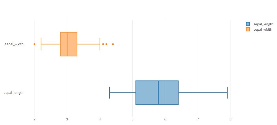
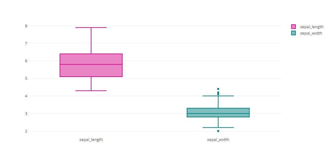
Boxplot

trace0 = go.Box(
    x=iris_data['sepal_length'],
    name='sepal_length'
)
trace1 = go.Box(
    x=iris_data['sepal_width'],
    name='sepal_width'
)
tmp = [trace0, trace1]
py.offline.iplot(tmp)

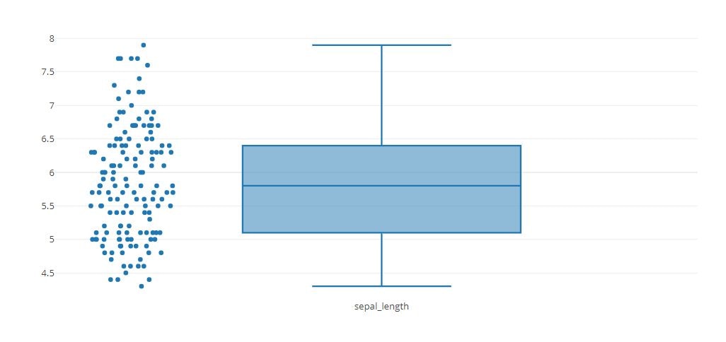
trace0 = go.Box(
    y=iris_data['sepal_length'],
    name='sepal_length',
    boxpoints='all', 
    jitter=0.3,
    pointpos=-1.8
)
tmp = [trace0]
py.offline.iplot(tmp)

trace0 = go.Box(
    y=iris_data['sepal_length'],
    name='sepal_length',
    marker = dict(
        color = 'rgb(214, 12, 140)',
    )
)
trace1 = go.Box(
    y=iris_data['sepal_width'],
    name='sepal_width',
    marker = dict(
        color = 'rgb(0, 128, 128)',
    )
)
tmp = [trace0, trace1]
py.offline.iplot(tmp)

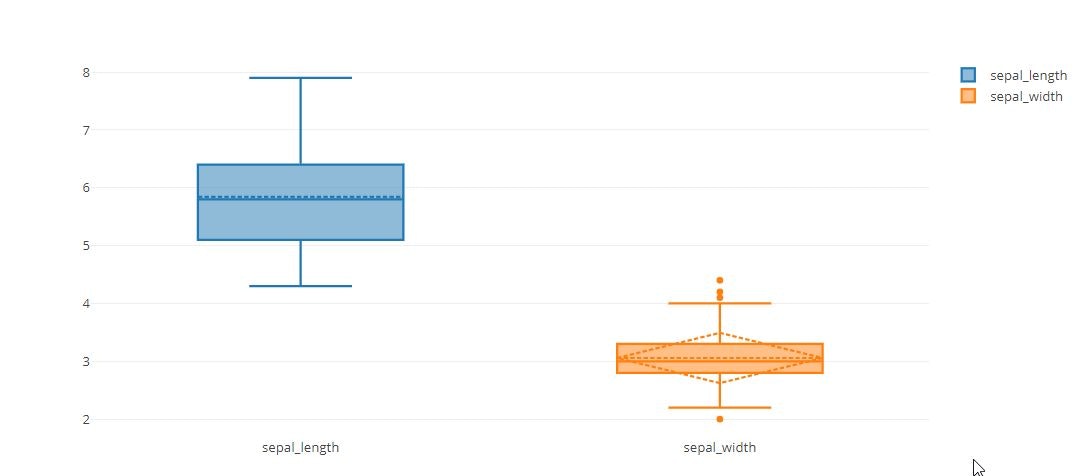
trace0 = go.Box(
    y=iris_data['sepal_length'],
    name='sepal_length',
    boxmean=True
)
trace1 = go.Box(
    y=iris_data['sepal_width'],
    name='sepal_width',
    boxmean='sd'
)
tmp = [trace0, trace1]
py.offline.iplot(tmp)

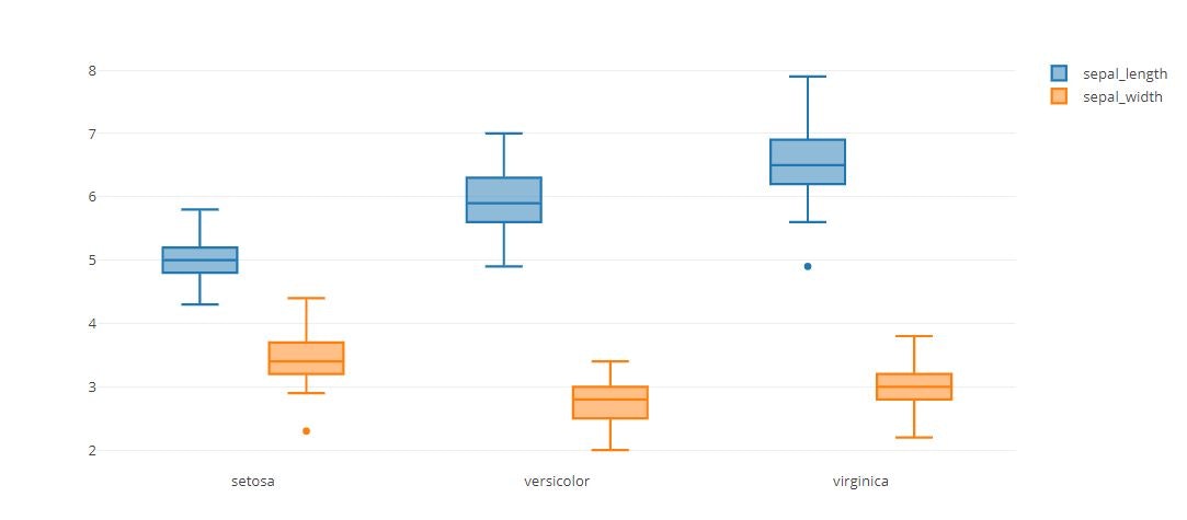
trace0 = go.Box(
    y=iris_data['sepal_length'],
    name='sepal_length',
    x=iris_data['species']
)
trace1 = go.Box(
    y=iris_data['sepal_width'],
    name='sepal_width',
    x=iris_data['species']
)
tmp = [trace0, trace1]
layout = go.Layout(
    boxmode='group'
)
fig = go.Figure(data=tmp, layout=layout)
py.offline.iplot(fig)

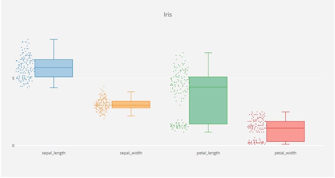
x_data = ['sepal_length', 'sepal_width',
          'petal_length', 'petal_width']
y0 = iris_data['sepal_length']
y1 = iris_data['sepal_width']
y2 = iris_data['petal_length']
y3 = iris_data['petal_width']

y_data = [y0,y1,y2,y3]

colors = ['rgba(93, 164, 214, 0.5)', 'rgba(255, 144, 14, 0.5)', 'rgba(44, 160, 101, 0.5)', 'rgba(255, 65, 54, 0.5)']

traces = []

for xd, yd, cls in zip(x_data, y_data, colors):
        traces.append(go.Box(
            y=yd,
            name=xd,
            boxpoints='all',
            jitter=0.5,
            whiskerwidth=0.2,
            fillcolor=cls,
            marker=dict(
                size=2,
            ),
            line=dict(width=1),
        ))

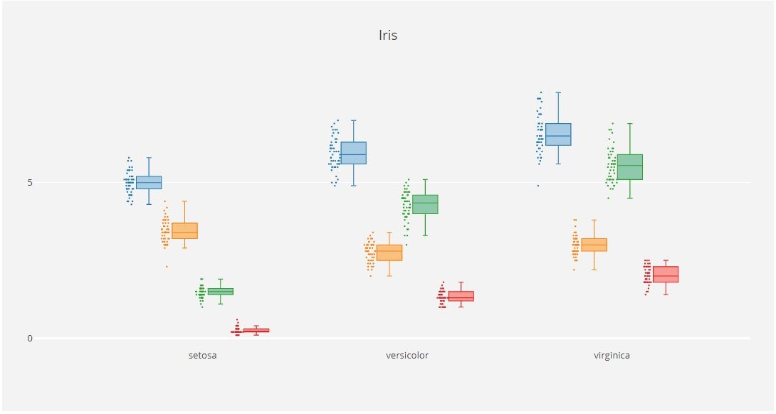
layout = go.Layout(
    title='Iris',
    yaxis=dict(
        autorange=True,
        showgrid=True,
        zeroline=True,
        dtick=5,
        gridcolor='rgb(255, 255, 255)',
        gridwidth=1,
        zerolinecolor='rgb(255, 255, 255)',
        zerolinewidth=2,
    ),
    margin=dict(
        l=40,
        r=30,
        b=80,
        t=100,
    ),
    paper_bgcolor='rgb(243, 243, 243)',
    plot_bgcolor='rgb(243, 243, 243)',
    showlegend=False
)

fig = go.Figure(data=traces, layout=layout)
py.offline.iplot(fig)

x_data = ['sepal_length', 'sepal_width',
          'petal_length', 'petal_width']
y0 = iris_data['sepal_length']
y1 = iris_data['sepal_width']
y2 = iris_data['petal_length']
y3 = iris_data['petal_width']

y_data = [y0,y1,y2,y3]

colors = ['rgba(93, 164, 214, 0.5)', 'rgba(255, 144, 14, 0.5)', 'rgba(44, 160, 101, 0.5)', 'rgba(255, 65, 54, 0.5)']

traces = []

for xd, yd, cls in zip(x_data, y_data, colors):
        traces.append(go.Box(
            y=yd,
            x=iris_data['species'],
            name=xd,
            boxpoints='all',
            jitter=0.5,
            whiskerwidth=0.2,
            fillcolor=cls,
            marker=dict(
                size=2,
            ),
            line=dict(width=1),
        ))

layout = go.Layout(
    title='Iris',
    yaxis=dict(
        autorange=True,
        showgrid=True,
        zeroline=True,
        dtick=5,
        gridcolor='rgb(255, 255, 255)',
        gridwidth=1,
        zerolinecolor='rgb(255, 255, 255)',
        zerolinewidth=2,
    ),
    margin=dict(
        l=40,
        r=30,
        b=80,
        t=100,
    ),
    paper_bgcolor='rgb(243, 243, 243)',
    plot_bgcolor='rgb(243, 243, 243)',
    showlegend=False,
    boxmode='group'
)

fig = go.Figure(data=traces, layout=layout)
py.offline.iplot(fig)

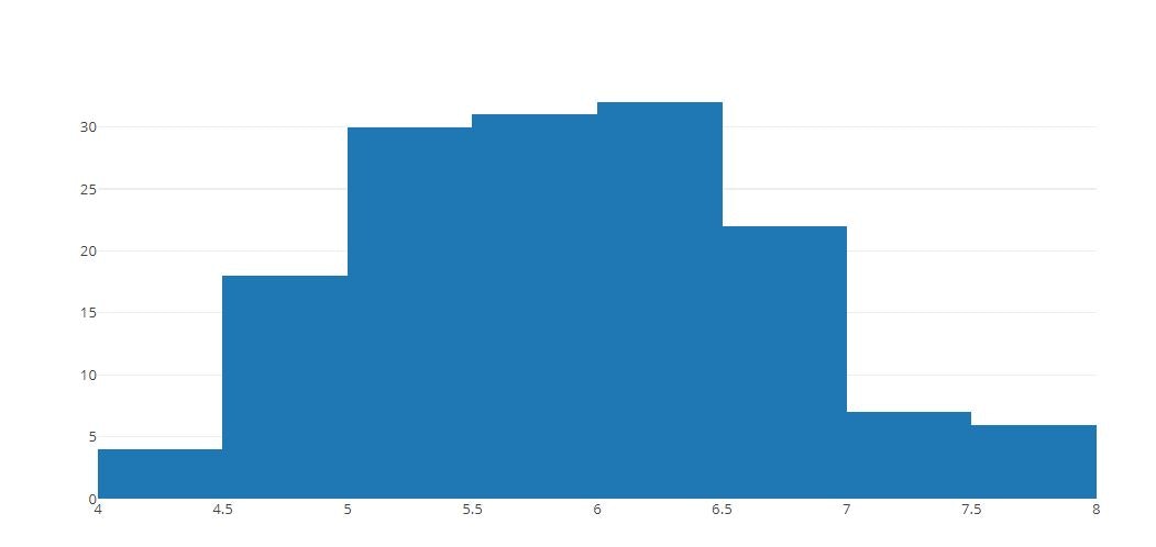
Histgram

# Basic Histogram
x = iris_data['sepal_length']
tmp = [go.Histogram(x=x)]

py.offline.iplot(tmp)

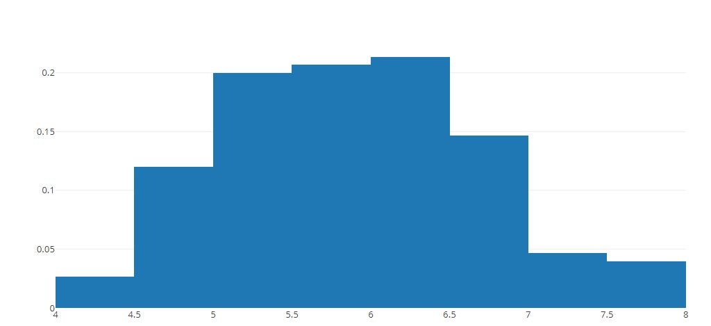
# Normalized Histogram
tmp = [go.Histogram(x=x,histnorm='probability')]

py.offline.iplot(tmp)

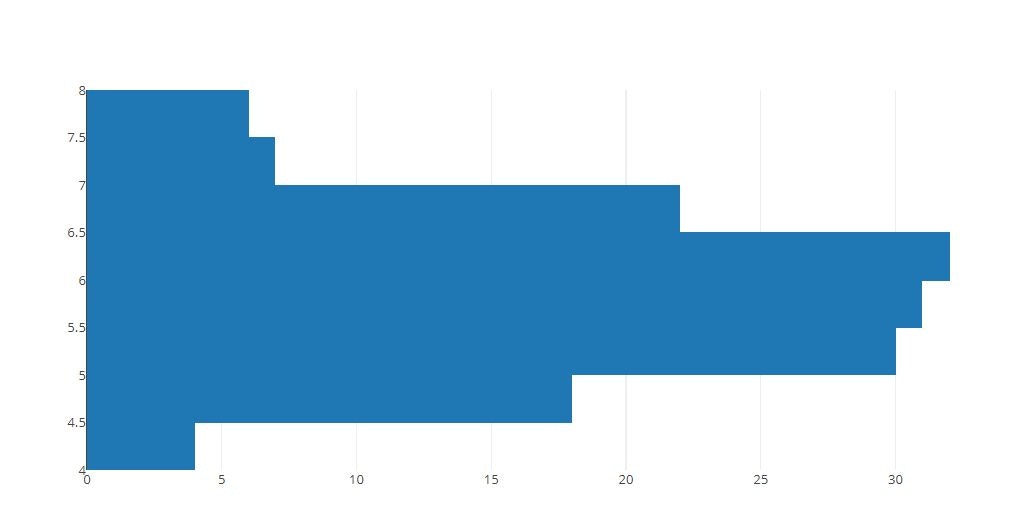
# Horizontal Histogram
tmp = [go.Histogram(y=x)]

py.offline.iplot(tmp)

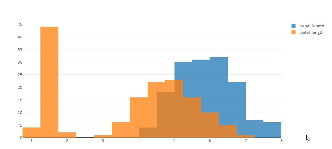
# Overlaid Histogram
x0 = iris_data['sepal_length']
x1 = iris_data['petal_length']

trace1 = go.Histogram(
    x=x0,
    opacity=0.75,
    name='sepal_length'
)
trace2 = go.Histogram(
    x=x1,
    opacity=0.75,
    name='petal_length'
)

tmp = [trace1, trace2]
layout = go.Layout(barmode='overlay')
fig = go.Figure(data=tmp, layout=layout)

py.offline.iplot(fig)

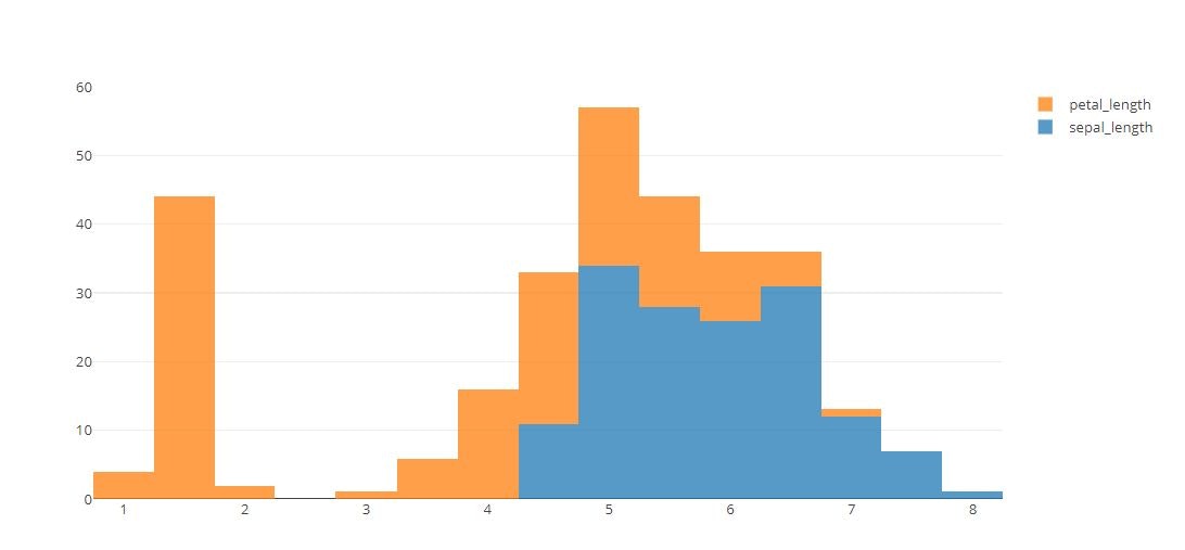
# Stacked Histograms
layout = go.Layout(barmode='stack')
fig = go.Figure(data=tmp, layout=layout)

py.offline.iplot(fig)

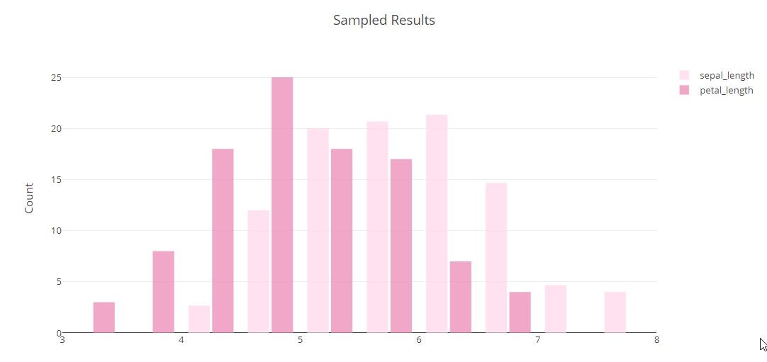
# Styled Histogram
x0 = iris_data['sepal_length']
x1 = iris_data['petal_length']

trace1 = go.Histogram(
    x=x0,
    histnorm='percent',
    name='sepal_length',
    xbins=dict(
        start=3.0,
        end=8.0,
        size=0.5
    ),
    marker=dict(
        color='#FFD7E9',
    ),
    opacity=0.75
)
trace2 = go.Histogram(
    x=x1,
    name='petal_length',
    xbins=dict(
        start=3.0,
        end=8.0,
        size=0.5
    ),
    marker=dict(
        color='#EB89B5'
    ),
    opacity=0.75
)
tmp = [trace1, trace2]

layout = go.Layout(
    title='Sampled Results',
    xaxis=dict(
        title='Value'
    ),
    yaxis=dict(
        title='Count'
    ),
    bargap=0.2,
    bargroupgap=0.1
)
fig = go.Figure(data=tmp, layout=layout)
py.offline.iplot(fig)

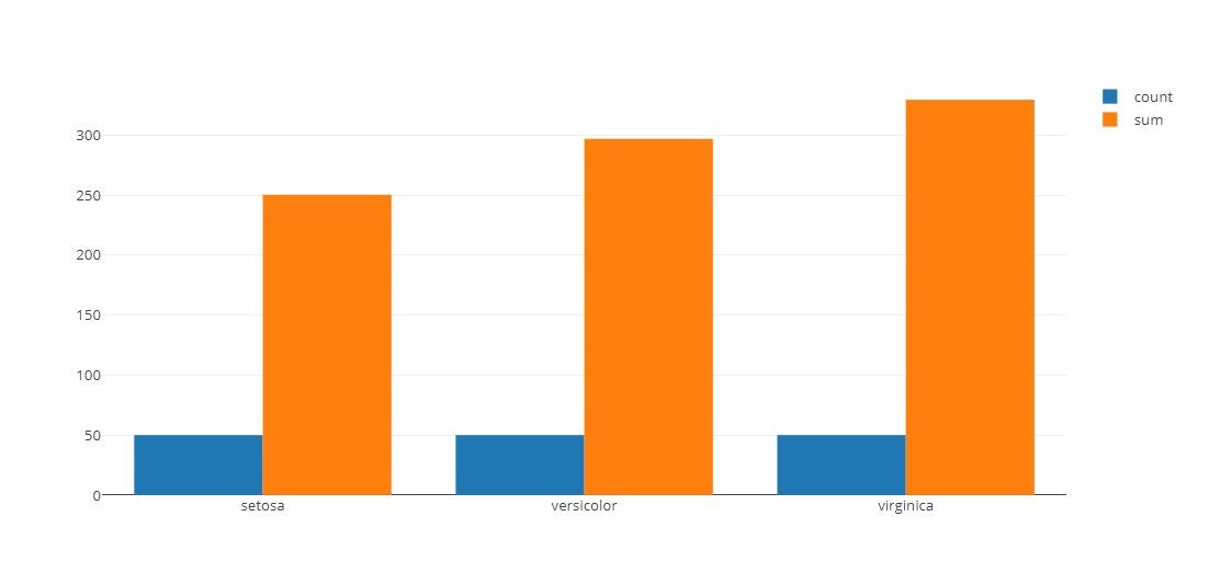
# Specify Binning Function
x = iris_data['species']
y = iris_data['sepal_length']

tmp = [
  go.Histogram(
    histfunc = "count",
    y = y,
    x = x,
    name = "count"
  ),
  go.Histogram(
    histfunc = "sum",
    y = y,
    x = x,
    name = "sum"
  )
]

py.offline.iplot(tmp)

2D Histogram

# 2D Histogram of a Bivariate Normal Distribution
x = iris_data['sepal_length']
y = iris_data['petal_length']

tmp = [
    go.Histogram2d(
        x=x,
        y=y
    )
]
py.offline.iplot(tmp)

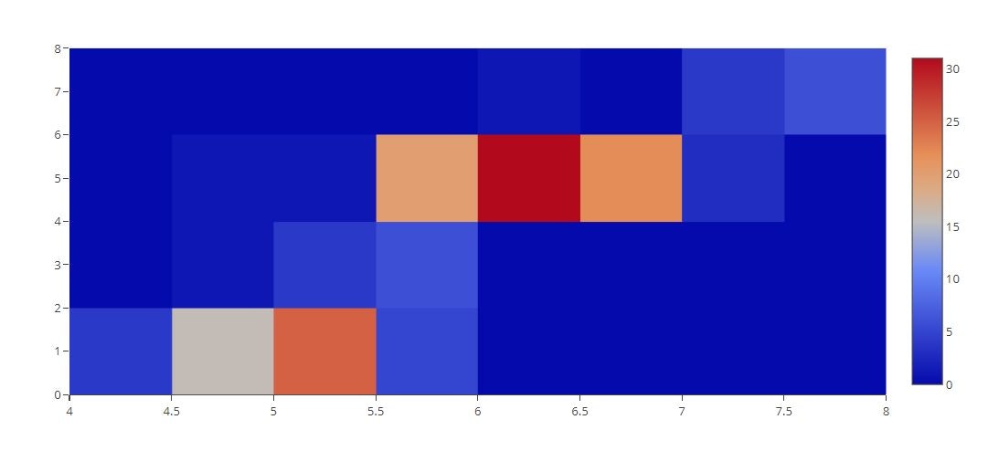
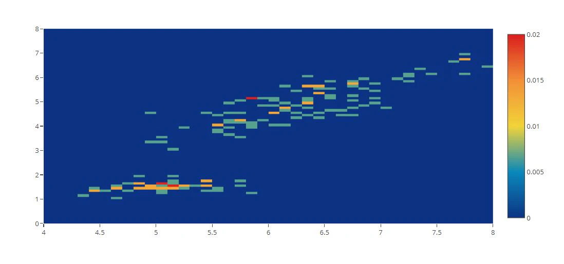
# 2D Histogram Binning and Styling Options
x = iris_data['sepal_length']
y = iris_data['petal_length']

tmp = [
    go.Histogram2d(x=x, y=y, histnorm='probability',
        autobinx=False,
        xbins=dict(start=4, end=8, size=0.1),
        autobiny=False,
        ybins=dict(start=0, end=8, size=0.1),
        colorscale=[[0, 'rgb(12,51,131)'], [0.25, 'rgb(10,136,186)'], [0.5, 'rgb(242,211,56)'], [0.75, 'rgb(242,143,56)'], [1, 'rgb(217,30,30)']]
    )
]
py.offline.iplot(tmp)

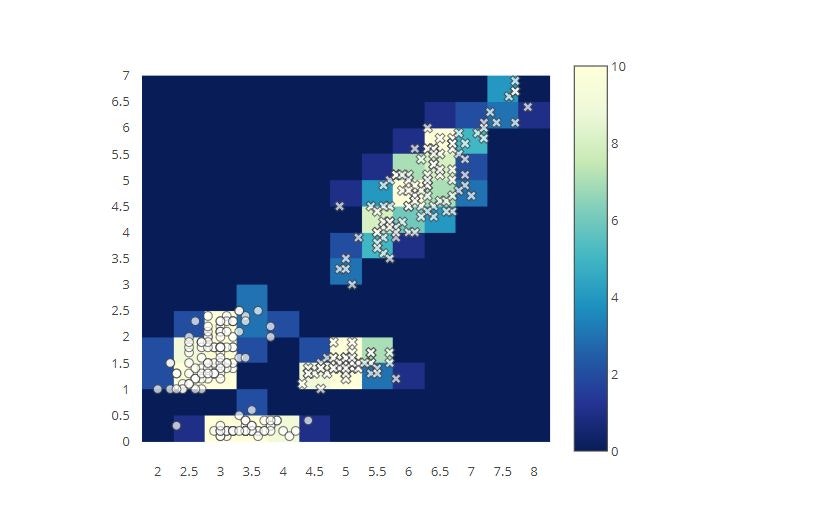
# 2D Histogram Overlaid with a Scatter Chart
x0 = iris_data['sepal_length']
y0 = iris_data['petal_length']
x1 = iris_data['sepal_width']
y1 = iris_data['petal_width']

x = np.concatenate([x0, x1])
y = np.concatenate([y0, y1])

trace1 = go.Scatter(
    x=x0,
    y=y0,
    mode='markers',
    showlegend=False,
    marker=dict(
        symbol='x',
        opacity=0.7,
        color='white',
        size=8,
        line=dict(width=1),
    )
)
trace2 = go.Scatter(
    x=x1,
    y=y1,
    mode='markers',
    showlegend=False,
    marker=dict(
        symbol='circle',
        opacity=0.7,
        color='white',
        size=8,
        line=dict(width=1),
    )
)
trace3 = go.Histogram2d(
    x=x,
    y=y,
    colorscale='YlGnBu',
    zmax=10,
    nbinsx=14,
    nbinsy=14,
    zauto=False,
)

layout = go.Layout(
    xaxis=dict( ticks='', showgrid=False, zeroline=False, nticks=20 ),
    yaxis=dict( ticks='', showgrid=False, zeroline=False, nticks=20 ),
    autosize=False,
    height=550,
    width=550,
    hovermode='closest',

)
tmp = [trace1, trace2, trace3]
fig = go.Figure(data=tmp, layout=layout)

py.offline.iplot(fig)

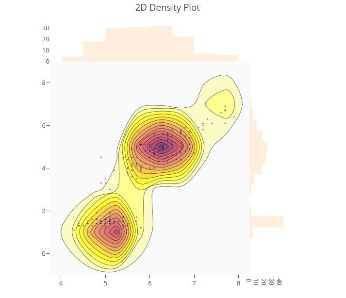
2D Density Plot

# 2D Histogram Contour Plot with Histogram Subplots
t = np.linspace(-1, 1.2, 2000)
x = iris_data['sepal_length']
y = iris_data['petal_length']

colorscale = ['#7A4579', '#D56073', 'rgb(236,158,105)', (1, 1, 0.2), (0.98,0.98,0.98)]

fig = ff.create_2d_density(
    x, y, colorscale=colorscale,
    hist_color='rgb(255, 237, 222)', point_size=3
)

py.offline.iplot(fig)

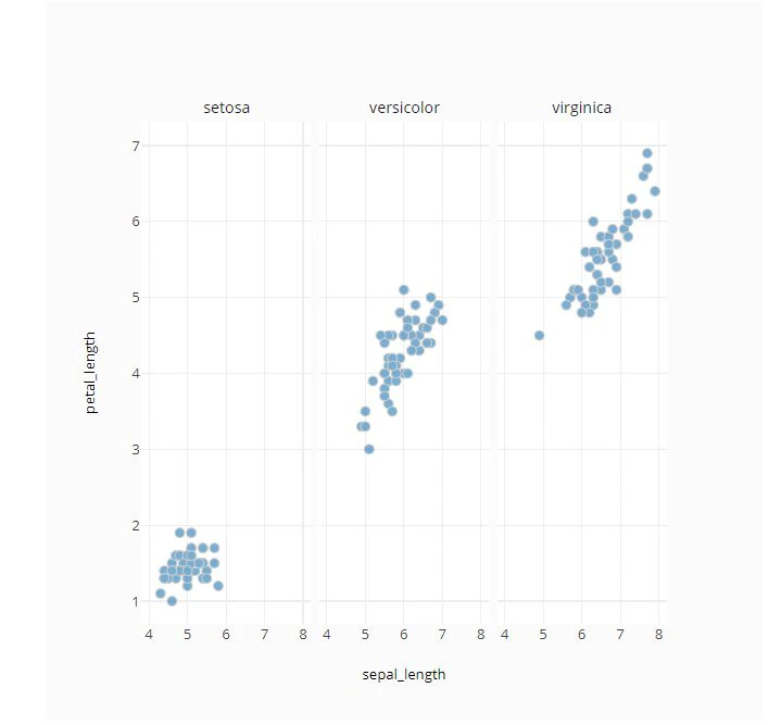
Facet and Trellis Plot

# Facet by Column
fig = ff.create_facet_grid(
    iris_data,
    x='sepal_length',
    y='petal_length',
    facet_col='species',
)

py.offline.iplot(fig)

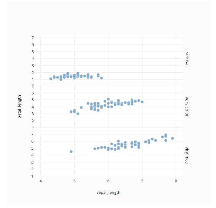
# Facet by Row
fig = ff.create_facet_grid(
    iris_data,
    x='sepal_length',
    y='petal_length',
    facet_row='species',
)

py.offline.iplot(fig)

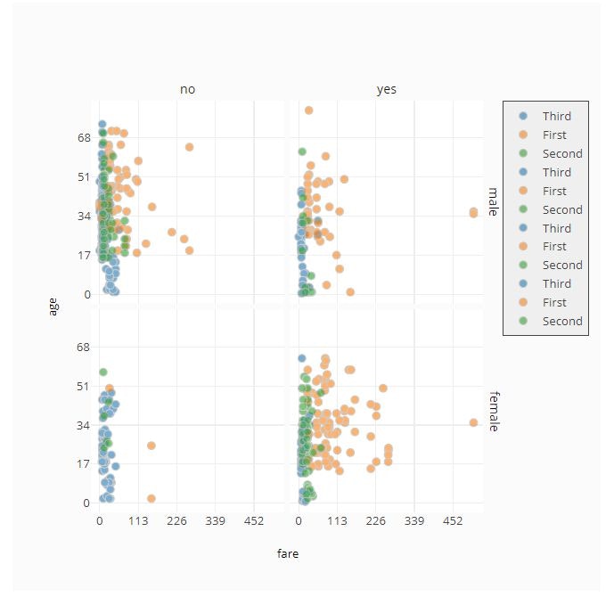
# Facet by Row and Column

fig = ff.create_facet_grid(
    titanic_data,
    x='fare',
    y='age',
    facet_row='sex',
    facet_col='alive',
    color_name='class',
    color_is_cat=True,
)

py.offline.iplot(fig)

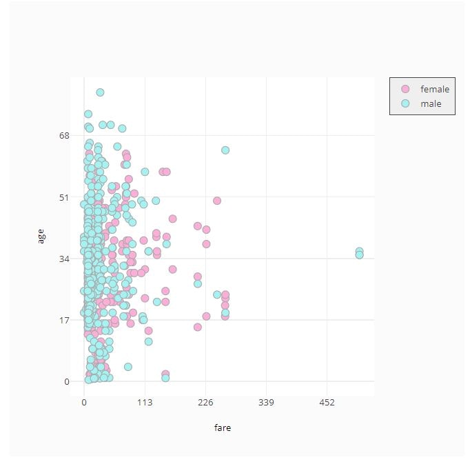
# Custom Colormap
fig = ff.create_facet_grid(
    titanic_data,
    x='fare',
    y='age',
    color_name='sex',
    show_boxes=False,
    marker={'size': 10, 'opacity': 1.0},
    colormap={'male': 'rgb(165, 242, 242)', 'female': 'rgb(253, 174, 216)'}
)
py.offline.iplot(fig)

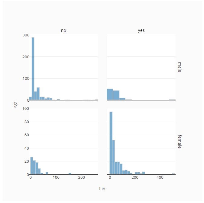
# Plot with Histogram Traces
fig = ff.create_facet_grid(
    titanic_data,
    x='fare',
    y='age',
    facet_row='sex',
    facet_col='alive',
    trace_type='histogram',
)

py.offline.iplot(fig)

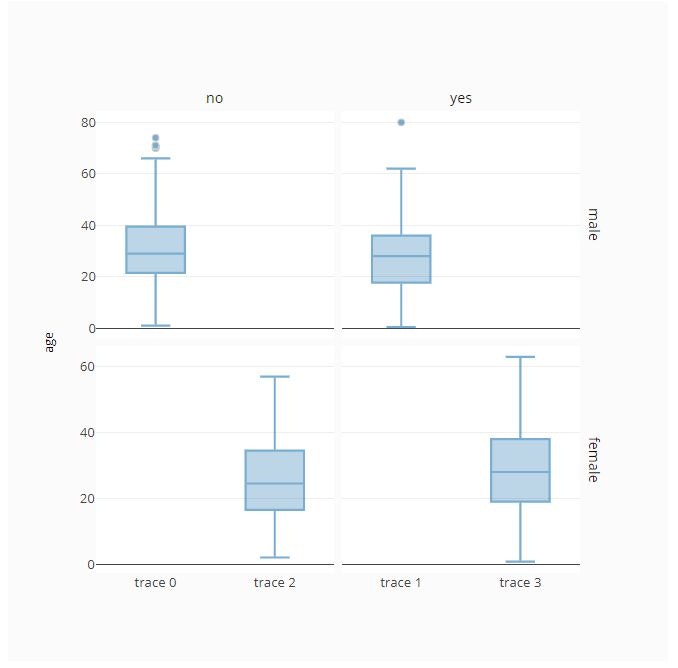
# Plot with BoxPlot Traces
fig = ff.create_facet_grid(
    titanic_data,
    y='age',
    facet_row='sex',
    facet_col='alive',
    trace_type='box',
)

py.offline.iplot(fig)

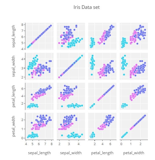
Scatterplot Matrix

classes=np.unique(iris_data['species'].values).tolist()
class_code={classes[k]: k for k in range(3)}
color_vals=[class_code[cl] for cl in iris_data['species']]
text=[iris_data.loc[ k, 'species'] for k in range(len(iris_data))]

pl_colorscale=[[0.0, '#19d3f3'],
               [0.333, '#19d3f3'],
               [0.333, '#e763fa'],
               [0.666, '#e763fa'],
               [0.666, '#636efa'],
               [1, '#636efa']]

trace1 = go.Splom(dimensions=[dict(label='sepal_length',
                                 values=iris_data['sepal_length']),
                            dict(label='sepal_width',
                                 values=iris_data['sepal_width']),
                            dict(label='petal_length',
                                 values=iris_data['petal_length']),
                            dict(label='petal_width',
                                 values=iris_data['petal_width'])],
                text=text,
                marker=dict(color=color_vals,
                            size=7,
                            colorscale=pl_colorscale,
                            showscale=False,
                            line=dict(width=0.5,
                                      color='rgb(230,230,230)'))
                )

axis = dict(showline=True,
          zeroline=False,
          gridcolor='#fff',
          ticklen=4)

layout = go.Layout(
    title='Iris Data set',
    dragmode='select',
    width=600,
    height=600,
    autosize=False,
    hovermode='closest',
    plot_bgcolor='rgba(240,240,240, 0.95)',
    xaxis1=dict(axis),
    xaxis2=dict(axis),
    xaxis3=dict(axis),
    xaxis4=dict(axis),
    yaxis1=dict(axis),
    yaxis2=dict(axis),
    yaxis3=dict(axis),
    yaxis4=dict(axis)
)

fig1 = dict(data=[trace1], layout=layout)
py.offline.iplot(fig1)

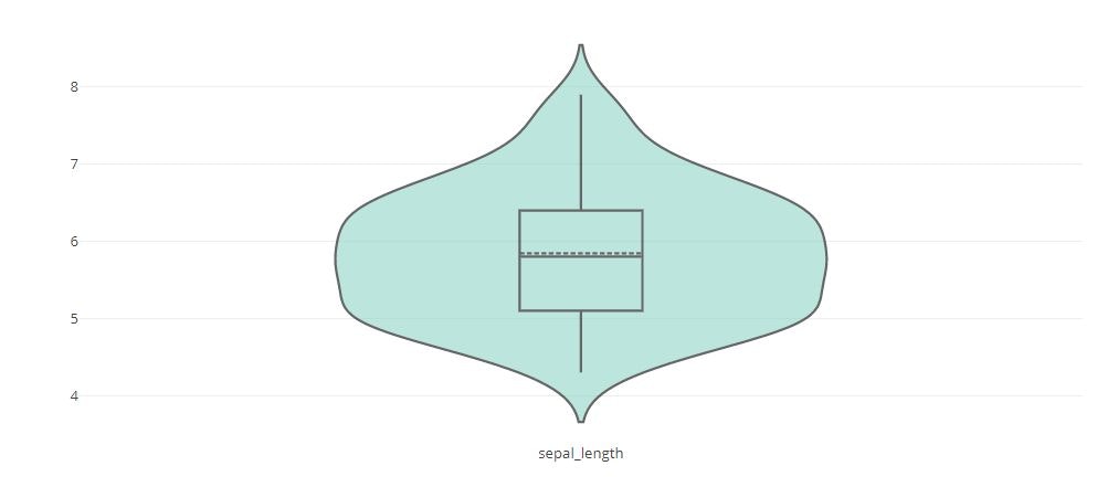
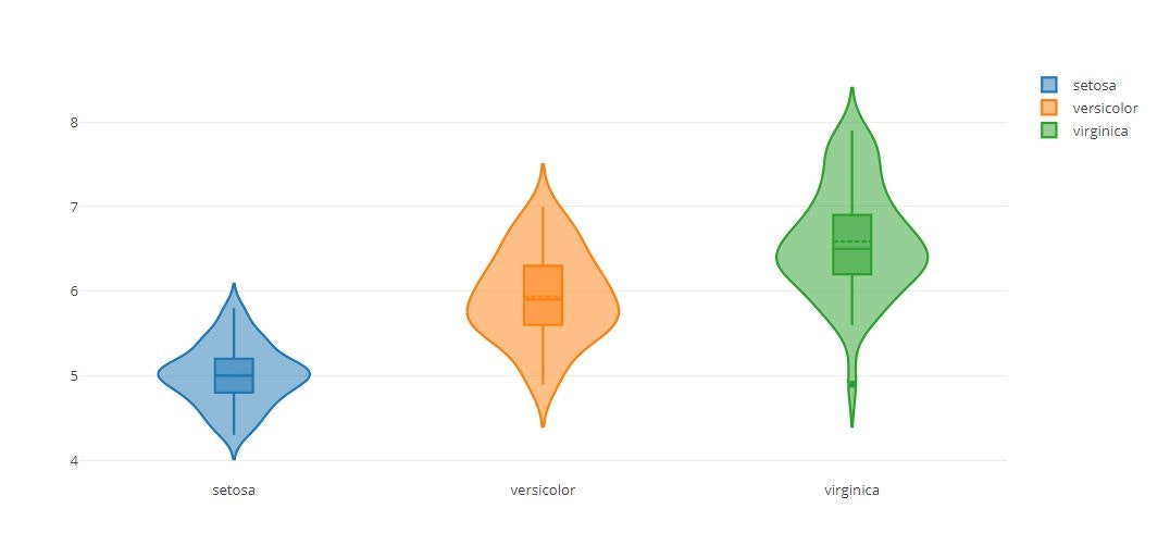
Violin Plot

# Basic Violin Plot
fig = {
    "data": [{
        "type": 'violin',
        "y": iris_data['sepal_length'],
        "box": {
            "visible": True
        },
        "line": {
            "color": 'black'
        },
        "meanline": {
            "visible": True
        },
        "fillcolor": '#8dd3c7',
        "opacity": 0.6,
        "x0": 'sepal_length'
    }],
    "layout" : {
        "title": "",
        "yaxis": {
            "zeroline": False,
        }
    }
}

py.offline.iplot(fig)

# Multiple Traces
tmp = []
for i in range(0,len(pd.unique(iris_data['species']))):
    trace = {
            "type": 'violin',
            "x": iris_data['species'][iris_data['species'] == pd.unique(iris_data['species'])[i]],
            "y": iris_data['sepal_length'][iris_data['species'] == pd.unique(iris_data['species'])[i]],
            "name": pd.unique(iris_data['species'])[i],
            "box": {
                "visible": True
            },
            "meanline": {
                "visible": True
            }
        }
    tmp.append(trace)


fig = {
    "data": tmp,
    "layout" : {
        "title": "",
        "yaxis": {
            "zeroline": False,
        }
    }
}

py.offline.iplot(fig)

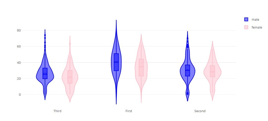
# Grouped Violin Plot
fig = {
    "data": [
        {
            "type": 'violin',
            "x": titanic_data['class'][ titanic_data['sex'] == 'male' ],
            "y": titanic_data['age'] [ titanic_data['sex'] == 'male' ],
            "legendgroup": 'male',
            "scalegroup": 'male',
            "name": 'male',
            "box": {
                "visible": True
            },
            "meanline": {
                "visible": True
            },
            "line": {
                "color": 'blue'
            }
        },
        {
            "type": 'violin',
            "x": titanic_data['class'][ titanic_data['sex'] == 'female' ],
            "y": titanic_data['age'] [ titanic_data['sex'] == 'female' ],
            "legendgroup": 'female',
            "scalegroup": 'female',
            "name": 'female',
            "box": {
                "visible": True
            },
            "meanline": {
                "visible": True
            },
            "line": {
                "color": 'pink'
            }
        }
    ],
    "layout" : {
        "yaxis": {
            "zeroline": False,
        },
        "violinmode": "group"
    }
}


py.offline.iplot(fig)

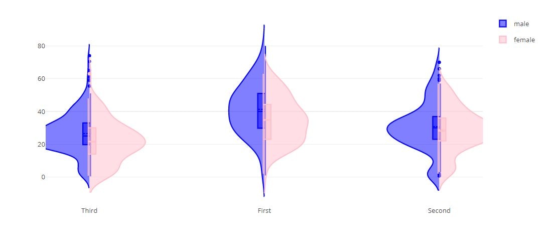
# Split Violin Plot
fig = {
    "data": [
        {
            "type": 'violin',
            "x": titanic_data['class'][ titanic_data['sex'] == 'male' ],
            "y": titanic_data['age'] [ titanic_data['sex'] == 'male' ],
            "legendgroup": 'male',
            "scalegroup": 'male',
            "name": 'male',
            "side": 'negative',
            "box": {
                "visible": True
            },
            "meanline": {
                "visible": True
            },
            "line": {
                "color": 'blue'
            }
        },
        {
            "type": 'violin',
            "x": titanic_data['class'][ titanic_data['sex'] == 'female' ],
            "y": titanic_data['age'] [ titanic_data['sex'] == 'female' ],
            "legendgroup": 'female',
            "scalegroup": 'female',
            "name": 'female',
            "side": 'positive',
            "box": {
                "visible": True
            },
            "meanline": {
                "visible": True
            },
            "line": {
                "color": 'pink'
            }
        }
    ],
     "layout" : {
        "yaxis": {
            "zeroline": False,
        },
        "violingap": 0,
        "violinmode": "overlay"
    }
}


py.offline.iplot(fig)

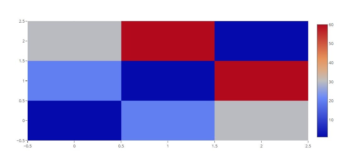
Heat Map

# Basic
trace = go.Heatmap(z=[[1, 20, 30],
                      [20, 1, 60],
                      [30, 60, 1]])
data=[trace]
py.offline.iplot(data)

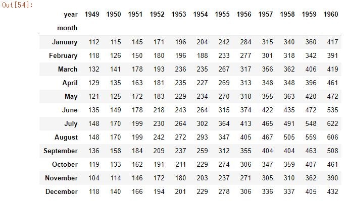
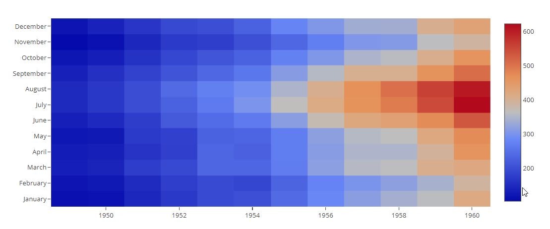
# Heatmap with Categorical Axis Labels
data = pd.pivot_table(data=flights_data, values='passengers', columns='year', index='month', aggfunc=np.mean)
data

trace = go.Heatmap(z=data.values,
                   x=data.columns,
                   y=data.index)
data=[trace]
py.offline.iplot(data)

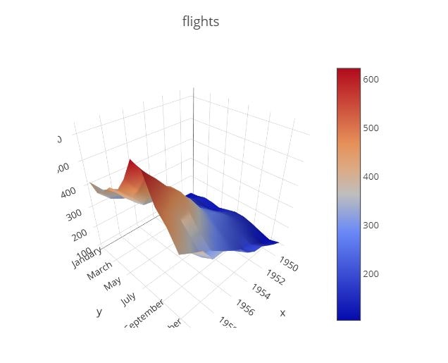
3D Surface

pivot_data = pd.pivot_table(data=flights_data, values='passengers', columns='year', index='month', aggfunc=np.mean)
data = [
    go.Surface(
        x=pivot_data.columns,
        y=pivot_data.index,
        z=pivot_data.values
    )
]
layout = go.Layout(
    title='flights',
    autosize=False,
    width=500,
    height=500,
    margin=dict(
        l=65,
        r=50,
        b=65,
        t=90
    )
)
fig = go.Figure(data=data, layout=layout)
py.offline.iplot(fig)

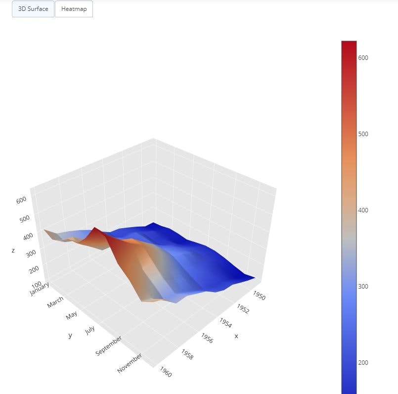
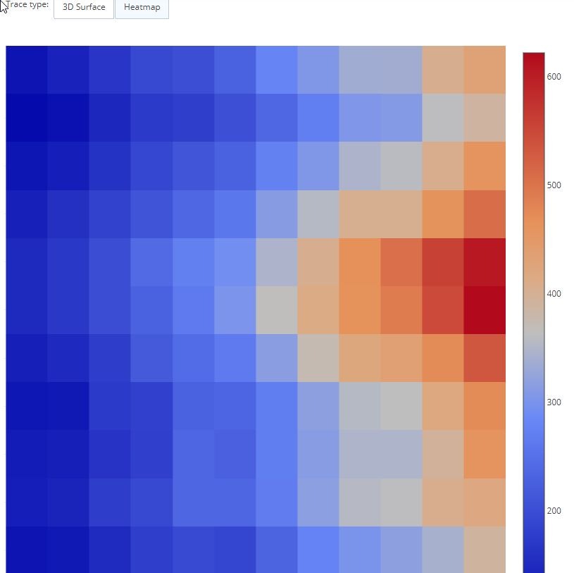
Restyle Button

pivot_data = pd.pivot_table(data=flights_data, values='passengers', columns='year', index='month', aggfunc=np.mean)
data = [
    go.Surface(
        x=pivot_data.columns,
        y=pivot_data.index,
        z=pivot_data.values
    )
]
layout = go.Layout(
    width=800,
    height=900,
    autosize=False,
    margin=dict(t=0, b=0, l=0, r=0),
    scene=dict(
        xaxis=dict(
            gridcolor='rgb(255, 255, 255)',
            zerolinecolor='rgb(255, 255, 255)',
            showbackground=True,
            backgroundcolor='rgb(230, 230,230)'
        ),
        yaxis=dict(
            gridcolor='rgb(255, 255, 255)',
            zerolinecolor='rgb(255, 255, 255)',
            showbackground=True,
            backgroundcolor='rgb(230, 230, 230)'
        ),
        zaxis=dict(
            gridcolor='rgb(255, 255, 255)',
            zerolinecolor='rgb(255, 255, 255)',
            showbackground=True,
            backgroundcolor='rgb(230, 230,230)'
        ),
        aspectratio = dict(x=1, y=1, z=0.7),
        aspectmode = 'manual'
    )
)

updatemenus=list([
    dict(
        buttons=list([   
            dict(
                args=['type', 'surface'],
                label='3D Surface',
                method='restyle'
            ),
            dict(
                args=['type', 'heatmap'],
                label='Heatmap',
                method='restyle'
            )             
        ]),
        direction = 'left',
        pad = {'r': 10, 't': 10},
        showactive = True,
        type = 'buttons',
        x = 0.1,
        xanchor = 'left',
        y = 1.1,
        yanchor = 'top' 
    ),
])

annotations = list([
    dict(text='Trace type:', x=1949, y=1.085, yref='paper', align='left', showarrow=False)
])
layout['updatemenus'] = updatemenus
layout['annotations'] = annotations

fig = dict(data=data, layout=layout)
py.offline.iplot(fig)

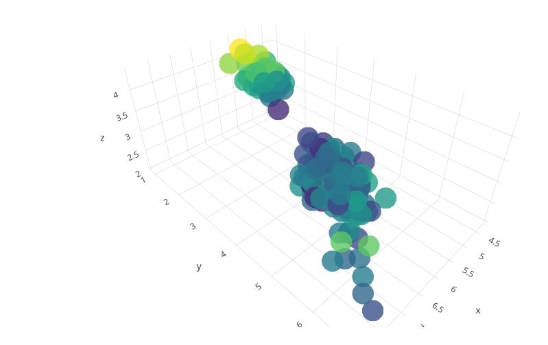
3D Scatter

trace1 = go.Scatter3d(
    x=iris_data['sepal_length'],
    y=iris_data['petal_length'],
    z=iris_data['sepal_width'],
    mode='markers',
    marker=dict(
        size=12,
        color=iris_data['sepal_width'],                # set color to an array/list of desired values
        colorscale='Viridis',   # choose a colorscale
        opacity=0.8
    )
)

data = [trace1]
layout = go.Layout(
    margin=dict(
        l=0,
        r=0,
        b=0,
        t=0
    )
)
fig = go.Figure(data=data, layout=layout)
py.offline.iplot(fig)

最後に

Plotlyは確かに綺麗なグラフが描けるんだけど、コーディングが結構煩雑になりやすい。
コーディングミスにも気を配る必要が出てくるから、特にこだわりが無いならSeaborn使った方が早いし無難かなと感じる。
会議とか見せ方を工夫したいときには、Plotly使うといいと思う。