はじめに
OpenFOAMから得られる圧力や流速などのデータを,paraViewを介さずにmatplotlibを使って2次元のコンター図として表示する方法についてまとめます。
解析の度にparaFoamを使ってコンター図に流線を追加したり,カラーバーを調整するのは時間がかかってしまいますので,postProcessコマンドのsurfaces を使って計算結果をVTK形式で出力させ,線上や面上のデータを取得してmatplotlibで表示させてみます。
実験した環境は以下の通りです。
- Ubuntu 18.04LTS
- OpenFOAM-v1912
- Python 3.6.9
- matplotlib 3.3.3
準備
VTKをPythonで扱うため,pip3を使ってインストールしておきます。
$ pip3 install vtk
データの用意
データとして,icoFoam のチュートリアルケース cavity を使います。
$ cp -r $FOAM_TUTORIALS/incompressible/icoFoam/cavity/cavity .
$ cd cavity
$ blockMesh
$ icoFoam
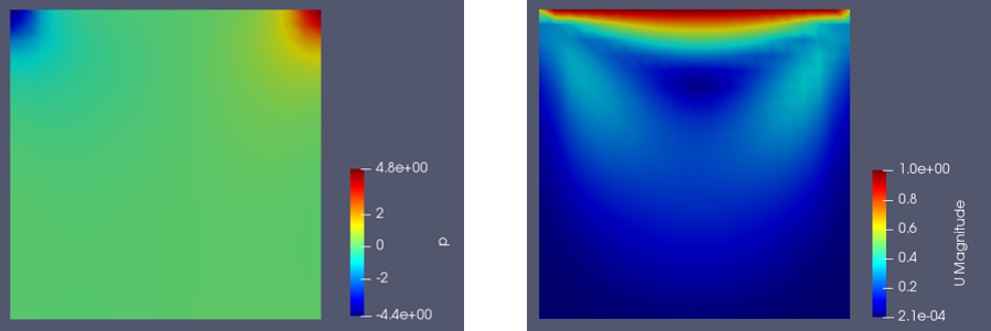
paraFoamを使って圧力と流速コンター図を描くとこんな感じになります。
データのサンプリングには postProcess コマンドの surfaces を使います。そのために system/surfaces を用意します。
/*--------------------------------*- C++ -*----------------------------------*\
  =========                 |
  \\      /  F ield         | OpenFOAM: The Open Source CFD Toolbox
   \\    /   O peration     | Website:  https://openfoam.org
    \\  /    A nd           | Version:  6
     \\/     M anipulation  |
-------------------------------------------------------------------------------
Description
    Writes out surface files with interpolated field data in VTK format, e.g.
    cutting planes, iso-surfaces and patch boundary surfaces.

    This file includes a selection of example surfaces, each of which the user
    should configure and/or remove.

\*---------------------------------------------------------------------------*/

# includeEtc "caseDicts/postProcessing/visualization/surfaces.cfg"

fields       (U p);
surfaceFormat  vtk;

surfaces
(
    xy
    {
        type                 plane;
        planeType            pointAndNormal;
        pointAndNormalDict
        {
            point       (0 0 0.005);
            normal    (0 0 1);
        }
    }
);

// ************************************************************************* //
fields で速度と圧力のデータを,surfaceFormat で vtk を指定しています。
平面のデータを取得するために,surfaces の type で plane を指定します。pointAndNormal は基準点と法線ベクトルの向きを指定します。
cavity のデータは z 軸方向に0.01の厚みがありますので,ここでは厚みの中心を通る xy 平面を抽出するように z=0.005 としています。
postProcess の実行
surfaces オプションをつけて実行します。
$ postProcess -func surfaces
$FOAM_RUN/cavity/postProcessing/surfaces の各時刻毎のディレクトリ内に vtp ファイルが作られます。
vtk と指定したはずなのに vtp 形式で出力されて焦りますが,落ち着いて vtk_to_numpy を使って読み込んでいきます。
matplotlib でコンター図出力
vtp 形式の polygon データを読み込む場合は vtkXMLPolyDataReader() を使います。
import numpy as np
import matplotlib.pyplot as plt
import matplotlib.cm as cm
import vtk
from vtk.util.numpy_support import vtk_to_numpy
from scipy.interpolate import griddata


filename = "postProcessing/surfaces/0.5/xy.vtp"

reader = vtk.vtkXMLPolyDataReader()
reader.SetFileName(filename)
reader.Update()
data = reader.GetOutput()

# cell data から point data変換
cell2point = vtk.vtkCellDataToPointData()
cell2point.SetInputData(reader.GetOutput())
cell2point.Update()

# 座標データの配列化
points = data.GetPoints()
coord = vtk_to_numpy(points.GetData()) # (x,y,z)座標の2次元配列
x = coord[:,0]
y = coord[:,1]
z = coord[:,2]

# メッシュグリッド用
xmin, xmax = min(x), max(x)
ymin, ymax = min(y), max(y)
xi = np.linspace(xmin, xmax, 100)
yi = np.linspace(ymin, ymax, 100)

# GetAbstractArray(0)は圧力、GetAbstractArray(1)は速度ベクトルデータ
p = vtk_to_numpy(cell2point.GetOutput().GetPointData().GetAbstractArray(0))
u = vtk_to_numpy(cell2point.GetOutput().GetPointData().GetAbstractArray(1))
speed = np.sqrt(u[:,0]**2 + u[:,1]**2) # ベクトルをスカラー値に変換

# 圧力のコンター図出力
levels = np.linspace(-5,5,21) # 描画する範囲の設定(最小,最大,色の分割数)
plt.tricontourf(x,y,p,levels=levels,cmap="jet",vmin=-5, vmax=5) #vmin,vmax で色の範囲を設定
cbar = plt.colorbar()
cbar.set_ticks(np.arange(-5,5.1,0.5)) # カラーバーの目盛り
cbar.set_label("p")
plt.show()

# 流速のコンター図出力
levels = np.linspace(0,1,21)
plt.tricontourf(x,y,speed,levels=levels,cmap="jet", vmin=0, vmax=1)
cbar = plt.colorbar()
cbar.set_ticks(np.arange(0,1.01,0.1))
cbar.set_label("U")
plt.show()
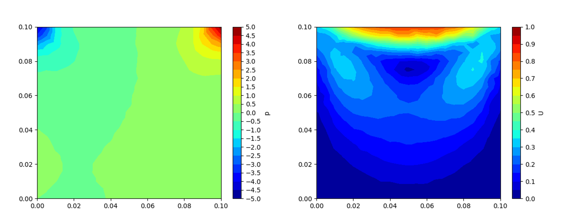
このスクリプトを実行して出力される圧力と流速グラフがこちら。
色の変化をもっと滑らかにしたい場合は,linspace の3つ目の引数を調整すると良いです。
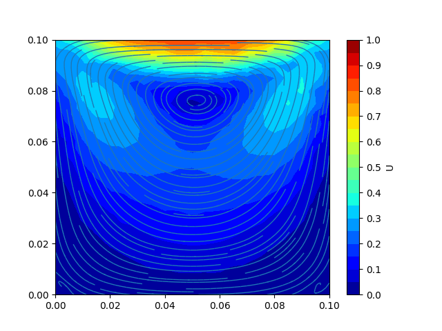
流線が必要な場合は streamplot() を使って描画することができます。
# 流線出力
levels = np.linspace(0,1,21)
velocity = griddata((x, y), u, (xi[None,:], yi[:,None]), method='linear') # 速度ベクトルをグリッドに合わせて線形補間
speed2 = np.sqrt(velocity[:,:,0]**2 + velocity[:,:,1]**2)
strm = plt.streamplot(xi, yi, velocity[:,:,0], velocity[:,:,1], linewidth=1, arrowstyle="-", density=1.5)
plt.tricontourf(x,y,speed,levels=levels,cmap="jet", vmin=0, vmax=1)
cbar = plt.colorbar()
cbar.set_ticks(np.arange(0,1.01,0.1))
cbar.set_label("U")
plt.show()
density で流線の密度,arrowstyle で矢印の形状を指定できます。
まとめ
同じケースで何度も計算をする場合,いちいちparaFoamを起動して操作する手間が省けるので便利です。
サクッとコンター図だけでも確認したい場合に重宝します。
以上です。