パラメータの最適化
実測データとモデルとの比較を行うとき、モデルの関数に含まれるパラメータの最適化は必須です。
大学に通っていた頃、自分の手でパラメータをちょっとずつ変えて最適化をしている努力家がいました。ソフトウェアが専門でない学科においては多少仕方のない光景ですが、やはりこういうのはプログラミングで解決しましょう。
今回紹介する2手法
- random search method (ランダムサーチ法)
- gradient descent method (最急降下法)
そもそもどのように最適化するのか
最適化プログラムの構成

これを何万回と繰り返し、最適なパラメータへと更新し続けます。
評価の仕方
最も一般的なのは、最小自乗法です。
今回の私のプログラムにも採用しています。
誤差をそのままではなく2乗してから足すことで、実測とモデルの誤差を積算することができます。
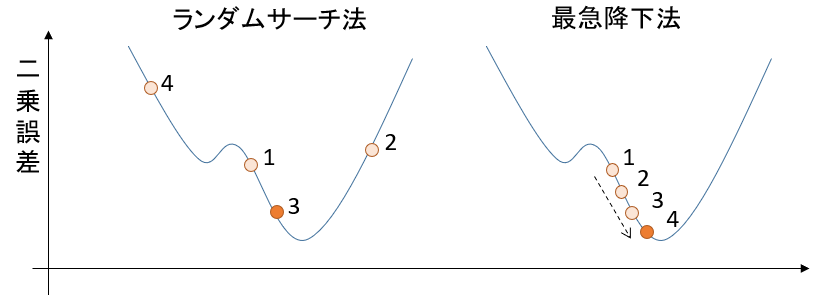
random search method (ランダムサーチ法)
パラメータにランダムな値を入れて,評価関数が一番小さくなる値を見つける手法です。
gradient descent method (最急降下法)
評価関数の偏微分値を求め、評価関数が小さくなる向きに少しずつパラメータをずらしていく手法です。
2手法の比較

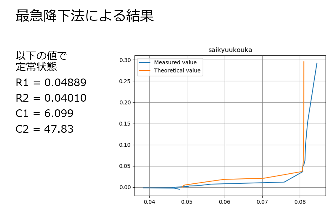
解の精度は、ランダムサーチ法 << 最急降下法
かなり精度に差があります。
ランダムサーチでは最適解に近づけば近づくほど、より最適なパラメータに近づくことが難しくなります。それに対して、最急降下法では堅実に最適解に近づくことができます。
ランダムサーチ法の試行回数をかなり増やしたとしても、再急降下法より良い精度を出すことはほぼ不可能でしょう。
参考程度に、4パラメータの最適化で10万回の試行回数でプログラムを回した結果を見てみましょう。
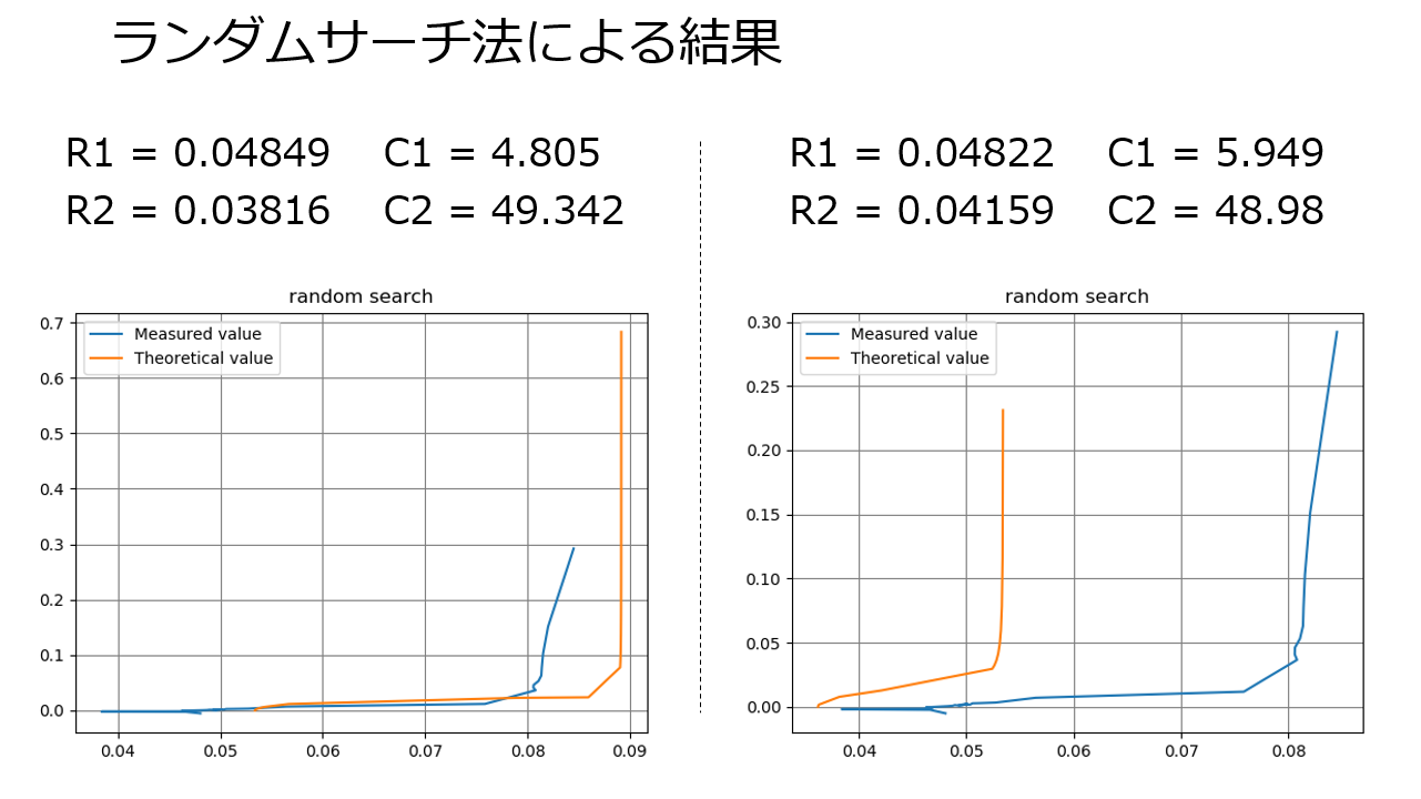
悲しいことに、10万回ランダムサーチしても、毎回答えが違うしグラフは全然沿いません。
精度面は、最急降下法の圧勝ですね。
最急降下法の欠点
そんな最急降下法にも致命的な欠点があります。
局所的な最適解にはまってしまうと、さらなる最適解があっても見つけられなくなるのです。
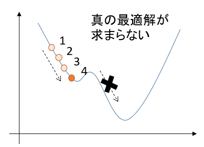
コンピュータに全てを委ねる最適化プログラムにおいて、「最適じゃない解」を出力する可能性があるのは見過ごせません。
2手法のコンビネーション
そこで、最も良い解決法が、「ランダムサーチ法と最急降下法のコンビネーション」です。
1. 大きな範囲を指定してランダムサーチをする。
2. 繰り返し行うことで最適な値があると推測される範囲を削っていく。
3. 最終的に、右に記した範囲になるまでランダムサーチを行う。
4. 最急降下法により最適解を求める。
これで問題解決です。
最後に、2手法のコード
実測値データは私が回路の周波数応答の計測をしたときのものです。
ランダムサーチ法
# random search method

import random
import numpy as np
import math
import matplotlib.pyplot as plt


# ----- data -----

freq = np.array([0.05, 0.1, 0.2, 0.4, 0.6061, 0.8, 1, 10,100])

ReR = np.array([0.005890792, 0.005824175, 0.005726238, 0.005501362, 0.005399829, 0.005244864, 0.0051687, 0.004736195, 0.004552081])

ImR = np.array([0.00476029, 0.002511934, 0.001470715, 0.000984505, 0.000808862, 0.000718529, 0.000655644, 0.00021882, -0.0000045569])

num=100000 # number of trials

# ----------------


lsv = 100000
Flist=[0 for i in range(num)]
R1list=[0 for i in range(num)]
R2list=[0 for i in range(num)]
C1list=[0 for i in range(num)]
C2list=[0 for i in range(num)]
N = len(freq)
R_opt = np.array([0j for i in range(N)])
theo = np.array([0j for i in range(N)])
R1_opt,R2_opt,C1_opt,C2_opt = 0,0,0,0


def init():
	sv = 0 # squares value
	R1 = random.uniform(0.001, 0.01)
	R2 = random.uniform(0.001, 0.01)
	C1 = random.uniform(0, 500)
	C2 = random.uniform(0, 500)
	return sv,R1,R2,C1,C2


def func_theoretical(R1,R2,C1,C2,freq):
	c1 = 1/(2j * math.pi * freq * C1)
	c2 = 1/(2j * math.pi * freq * C2)
	c3 = R2 + c2
	theo = R1 + c1*c3/(c1+c3)
	return theo


def func_distance(ReR, ImR, theo):
	return (ReR - theo.real) **2 + (ImR + theo.imag) **2


# --- traials ---
for i in range(num):
	sv,R1,R2,C1,C2 = init()

	for i in range(N):
		theo[i] = func_theoretical(R1,R2,C1,C2,freq[i])
		sv += func_distance(ReR[i], ImR[i], theo[i])

	if sv < lsv:
		lsv = sv
		R_opt = theo
		R1_opt,R2_opt,C1_opt,C2_opt = R1,R2,C1,C2
# ----------------


# --- result ---
print('number of trials :',num)
print('Least Squares Value :',lsv)
print('R1,R2,C1,C2 :' ,R1_opt,R2_opt,C1_opt,C2_opt)


# --- graph ---
plt.title('random search', loc='center')
plt.plot(ReR,ImR, label="Measured value")
plt.plot(R_opt.real, - R_opt.imag ,label="Theoretical value")
plt.grid(color='gray')
plt.legend(loc="upper left")
plt.show()
最急降下法
import random
import numpy as np
import math
import matplotlib.pyplot as plt


# --- data ---

freq = np.array([0.05, 0.1, 0.2, 0.4, 0.6061, 0.8, 1, 10,100])

ReR = np.array([0.005890792, 0.005824175, 0.005726238, 0.005501362, 0.005399829, 0.005244864, 0.0051687, 0.004736195, 0.004552081])

ImR = np.array([0.00476029, 0.002511934, 0.001470715, 0.000984505, 0.000808862, 0.000718529, 0.000655644, 0.00021882, -0.0000045569])

# ------------


# --- setting ---

ParaList = [0.005, 0.0014, 138 , 546] #R1,R2,C1,C2

d = [0.00001, 0.000001, 0.1, 0.1] #d(R1,R2,C1,C2)

num=1000 # number of trials
pf=11 # print freqency

# ----------------

def func_lsv():
	global freq, ReR, ImR, ParaList

	R1,R2,C1,C2 = ParaList
	for Freq, rer, imr in zip(freq, ReR, ImR):
		a = 1/(2j * math.pi * freq * C1)
		b = 1/(2j * math.pi * freq * C2)
		c = R2 + b
		R = R1 + a*c/(a+c)
		distance = (ReR - R.real) **2  + (ImR + R.imag) **2
	lsv = sum(distance)
	return lsv


def gradient_descent(N,Rs):
	global ParaList

	ParaList[N] = ParaList[N] - Rs
	lsv_under = func_lsv()
	ParaList[N] = ParaList[N] + 2 * Rs
	lsv_over = func_lsv()

	if lsv_under < lsv_over :
		ParaList[N] = ParaList[N] - 2 * Rs
		lsv = lsv_under
	else:
		lsv = lsv_over

	return ParaList, lsv


# --- main ---
cnt_pf=0
print("  R1  /  R2  /  C1  /  C2  /  Least Squares Value")

for i in range(num):
	cnt_pf +=1
	for N in range(4):
		ParaList, lsv = gradient_descent(N, d[N])
	if cnt_pf == pf:
		print(ParaList,lsv)
		cnt_pf=0


Rbest=np.array([0j for i in range(len(freq))])

R1,R2,C1,C2 = ParaList
for i in range(len(freq)):
	a = 1/(2j * math.pi * freq[i] * C1)
	b = 1/(2j * math.pi * freq[i] * C2)
	c = R2 + b
	Rbest[i] = R1 + a*c/(a+c)


# --- result ---
print('trials :',num)
print('Least Squares Value: :', lsv)
print('R1 ,R2, C1, C2 :',ParaList)


# --- graph ---
plt.title('saikyuukouka', loc='center')
plt.plot(ReR,ImR, label="Measured value")
plt.plot(Rbest.real, -Rbest.imag ,label="Theoretical value")
plt.grid(color='gray')
plt.legend(loc="upper left")
plt.show()