Excelに整理した「アンケート自由記述」を分析しよう！（その2）〜TF-IDFで分類編〜

はじめに

前回の記事では、
Excelに整理した「アンケート自由記述」の自然言語分析 をやってみました。
主には、語彙のカウント、ベクトル化などを通じ、可視化するというものですが、これで「Userが自由記述で何を訴えようとしているか？」がはっきりするわけではありません。
可視化した結果を真摯に眺め、KJ法的にいうならば、Userの訴えかけに耳を傾けなければいけません。
「すべてのUserの訴えかけに目を通すぞ」という心意気も大切ですが、Userの訴えかけにはどのようなバリエーションがあるのか？を把握したうえで、臨めた方がよいでしょう。
ではどんなバリエーションの見方があるでしょうか？
『満足度によってUserの訴えかけに違いがあるか？』は、やりやすく、わかりやすい見方のひとつだと思います。
満足度の高いUser、低いUserの訴えかけに違いを見いだすことができれば、改善につなげられる可能性を高めることができます。

ただ、

• 満足度の高いUserの訴えは建設的？
• 満足度の低いUserの訴えは否定的？
• 満足度に限らず、同じ訴えをもつUserもおられるのでは？

Userには率直な方、天の邪鬼な方、いろいろおられますので、こればかりは仕方がありませんが、アンケート数が少ない場合は、満足度の傾向だけで語るのは危険かもしれません。

そこで、
Userの訴えかけの傾向の違いを、語彙の傾向でわけらられないか？がこの記事のテーマです。

Userの訴えかけの違いでグループわけができると、バリエーション全体を眺めたなかで、個々のUserの訴えかけに向きあうことができ、より効率的に自由記述の内容が理解できるようになると思います。

実行条件など

・Google colabで実行
・手元の表形式データ（アンケート自由記述結果）で実行
※使用したデータは開示できませんが、データ形式は以下です。カラムはUserID、comment、csの3つ。commentは自由記述回答、csは満足度（1～6）です。

userID	comment	cs
U001	総合的には満足してますが、○○が細かく調整できたらもっと使いやすいと思います。	4
U002	○○ボタンが押しにくいです。	2
U003	特にありません。	3
U004	既存品と取付位置が合わないことがつらいです。	1

語彙のベクトル化について

Userの訴えかけを語彙傾向で分けるためには、語彙をベクトル化しないといけません。
私はTF-IDF、word2vec、Doc2Vecを試しました。
この記事では、TF-IDFによる方法を扱っています。
各Userの声、形態素の結果、グループ分け（クラスタ分け）の結果をデータフレームに格納、csvデータに変換し、ローカルファイルに出力するようにしています。
グループ分けした結果は、EXCELで並べ替えるなどして見たほうがよいでしょう。

備忘

• 実行内容は前回の記事がベース。
• コード操作を不要にするため、ファイル指定やフォームなど、GoogleColabの機能を活用。
• 品詞は名詞・動詞・形容詞（動詞と形容詞は基礎型）を抽出対象とした。
• 分かち書きは、スペース区切り（語A 語B 語C）とカンマ区切り [語A,語B,語C] の2パターン。TF-IDF計算はスペース区切り、Word Cloudは カンマ区切り、nlplotはどちらでもいけたと思います。（※1パターンだけで対応したかったが…私の修行が足りないのだと思います。）

ライブラリのインストール

nlplotをインストール

pip install nlplot

日本語フォント

#日本語フォントをインストール
!apt-get -y install fonts-ipafont-gothic

MeCabのインストール

#Mecabのインストール
!pip install mecab-python3==0.996.5

matplotlib日本語化

#matplotlib日本語化
!pip install japanize-matplotlib

ライブラリインポート

from pathlib import Path
import pandas as pd
import re
import MeCab
import matplotlib.pyplot as plt
import warnings
warnings.filterwarnings('ignore')

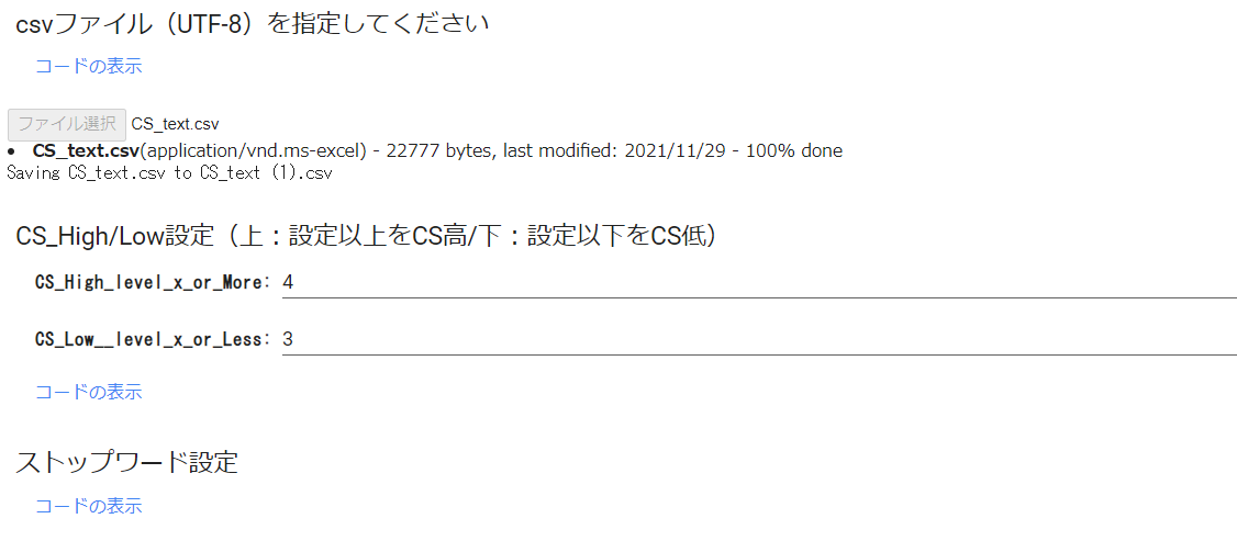
ファイル & CS_High/Low_Level & ストップワード指定

※CSは顧客満足度です。

#@title csvファイル（UTF-8）を指定してください
from google.colab import files
#print('csvファイル(UTF-8）を指定してください')
uploaded = files.upload()

#@title CS_High/Low設定（上：設定以上をCS高/下：設定以下をCS低） { run: "auto" }
CS_High_level_x_or_More = 4 #@param {type:"number"}
CS_Low__level_x_or_Less = 3 #@param {type:"number"}

#@title ストップワード設定
stop_words = ["し", "い", "ある", "おる", "せる", "ない", "いる", "する", "の", "よう", "なる", "それ", "そこ", "これ", "こう", "ため", "そう", "れる", "られる"]

※GoogleColabのフォームを使うと表示は以下のようになります。

モジュール構築

#@title データフレーム格納＆欠損値削除
if len(uploaded.keys()) != 1:
    print("アップロードは１ファイルにのみ限ります")
else:
    target = list(uploaded.keys())[0]

df = pd.read_csv(target)

df.dropna(subset=['comment'], inplace=True)
df.head()

#@title 形態素解析（一般名詞・動詞:基礎型・形容詞:基礎型）＆カンマ･スペース区切りをデータフレームに格納
#形態素解析（一般名詞・動詞・形容詞（動詞と形容詞は基礎型）を抽出対象とした）
#スペース区切り分かち書き
def mecab_analysis(text):

    t = MeCab.Tagger('-Ochasen')

    node = t.parseToNode(text)

    words = []

    while node:
        if node.surface != "":  # ヘッダとフッタを除外

            word_type = node.feature.split(',')[0]
            sub_type = node.feature.split(',')[1]
            features_ = node.feature.split(',')

            #品詞を選択
            if word_type in ["名詞"]: 
#                if sub_type in ['一般']:
                    word = node.surface
                    words.append(word)

            #動詞、形容詞[基礎型]を抽出（名詞のみを抽出したい場合は以下コードを除く）
            elif word_type in ['動詞','形容詞'] and not (features_[6] in stop_words):
                words.append(features_[6])

        node = node.next

        if node is None:
            break

    return " ".join(words)

#カンマ区切り分かち書き
def mecab_analysis2(text):

    t = MeCab.Tagger('-Ochasen')

    node = t.parseToNode(text)

    words2 = []

    while(node):

        if node.surface != "":  # ヘッダとフッタを除外
            word_type = node.feature.split(',')[0]
            sub_type = node.feature.split(',')[1]
            features_ = node.feature.split(',')

            if word_type in ['名詞']: #名詞をリストに追加する
#                if sub_type in ['一般']:
                    words2.append(node.surface)

            #動詞、形容詞[基礎型]を抽出（名詞のみを抽出したい場合は以下コードを除く）
            elif word_type in ['動詞','形容詞'] and not (features_[6] in stop_words):
                    words2.append(features_[6])

        node = node.next
        if node is None:
            break
    return words2

#形態素結果をリスト化し、データフレームdf1に結果を列追加する
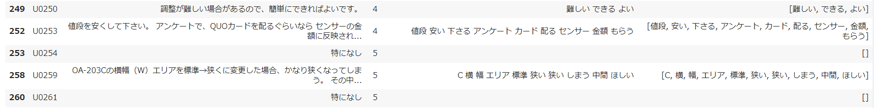
df['words'] = df['comment'].apply(mecab_analysis)
df['words2'] = df['comment'].apply(mecab_analysis2)

#表示
df

※表示の一部抜粋

#@title 形態素結果を層別しデータフレームに格納
#全データをデータフレームに格納
all_words=' '.join(df['words'])
df_all = pd.Series(all_words)

#CSが高いuserの声（words）をデータフレームに格納
drop_index = df.index[df['cs'] <=CS_Low__level_x_or_Less]
#条件にマッチしたIndexを削除
df_high = df.drop(drop_index)
all_high_words=' '.join(df_high['words'])
df_all_high_words = pd.Series(all_high_words)

#CSが低いuserの声（words）をデータフレームに格納
drop_index2 = df.index[df['cs'] >=CS_High_level_x_or_More]
#条件にマッチしたIndexを削除
df_low = df.drop(drop_index2)
all_low_words=' '.join(df_low['words'])
df_all_low_words = pd.Series(all_low_words)

print('CS高ユーザーの声(Words）：')
print(df_all_high_words)
print('CS低ユーザーの声(Words）：')
print(df_all_low_words)

#@title ワード出現回数カウント（表示する場合は#外す）
#カンマ区切り分かち書きしたワードをリスト化
words_list = df.words2.tolist()
words_list = sum(words_list,[])

from collections import Counter

#出現回数を集計し、最頻順にソートし、resultに格納
words_count = Counter(words_list)
result = words_count.most_common()

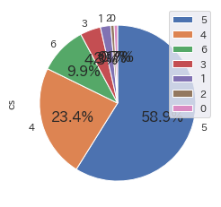
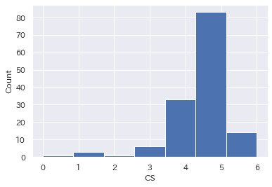
#@title CS満足度傾向_円グラフ & ヒストグラム
cs = pd.DataFrame(df['cs'].value_counts())
cs.plot.pie(subplots=True,autopct="%1.1f%%",startangle=90,counterclock=False)
plt.show()

plt.hist(df['cs'],bins=7)
# x軸とy軸のラベルをつける
plt.xlabel('CS')
plt.ylabel('Count')
plt.show()

nlpot

#@title uni-gram表示
import nlplot

npt = nlplot.NLPlot(df, target_col='words')

# top_nで頻出上位単語, min_freqで頻出下位単語を指定できる
#stopwords = npt.get_stopword(top_n=0, min_freq=0)

npt.bar_ngram(
    title='uni-gram',
    xaxis_label='word_count',
    yaxis_label='word',
    ngram=1,
    top_n=50,
#    stopwords=stopwords,
)

#@title tree map表示
npt.treemap(
    title='Tree of Most Common Words',
    ngram=1,
    top_n=30,
#    stopwords=stopwords,
)

#@title Word Cloud表示（nlpot）
npt.wordcloud(
    max_words=100,
    max_font_size=100,
    colormap='tab20_r',
#    stopwords=stopwords,
)

#@title Word Distribution表示（単語数の分布）
# 単語数の分布
npt.word_distribution(
    title='number of words distribution',
    xaxis_label='count',
)

#@title Build Graph（共起ネットワーク）表示
# ビルド（データ件数によっては処理に時間を要します）※ノードの数のみ変更
npt.build_graph(min_edge_frequency=1,
                #stopwords=stopwords,
                )

display(
    npt.node_df.head(), npt.node_df.shape,
    npt.edge_df.head(), npt.edge_df.shape
)

npt.co_network(
    title='Co-occurrence network',
)

#@title Sunburst表示
npt.sunburst(
    title='All sentiment sunburst chart',
    colorscale=True,
    color_continuous_scale='Oryel',
    width=800,
    height=600,
    #save=True
)

Word Cloud

• ワードクラウドは、文章中で出現頻度が高い語を複数選び出し、その頻度に応じた大きさで図示する手法。
• 表示するワードクラウドは全4種。①ワード出現回数ベース／②TF-IDFベース（全データ）/③TF-IDFベース（CS高データ）/④TF-IDFベース（CS低データ）\ ※語の表示数はmax_words, Word Cloudの表示サイズはwidth, heightで設定できる

TF-IDF
- TF-IDF は文書に含まれる単語がどれだけ重要かを示す手法の一つで、TF (= Term Frequency: 単語の出現頻度)と IDF (Inverse Document Frequency: 逆文書類度)の2つを使って計算します。

#@title TF-IDFマトリクス作成＆データフレーム格納
# ライブラリインポート
from sklearn.feature_extraction.text import TfidfVectorizer

# TF-IDFのベクトル処理
vectorizer = TfidfVectorizer(use_idf=True)
tfidf = vectorizer.fit_transform(df['words'] )

# TF-IDF値を「センテンス×ワード」マトリクスをデータフレーム化
df_tfidf = pd.DataFrame(tfidf.toarray(), columns=vectorizer.get_feature_names(), index=df['words'])
#display(df_tfidf)

#@title Word Cloud by word_count（All Data）：🔲型 → #maskの#外すと🍩型に

#wordcloud取込用にresultを辞書型ヘ変換
dic_result = dict(result)

#Word Cloudで画像生成（#max_words, width, heightは任意設定）
from wordcloud import WordCloud

#画像データダウンロード（biwakoの画像リンクもあり。変更する場合は#調整）
import requests

url = "https://github.com/hima2b4/Word-Cloud/raw/main/donuts.png"
#url = "https://github.com/hima2b4/Word-Cloud/raw/main/biwa.png"

file_name = "donuts.png"
#file_name = "biwa.png"

response = requests.get(url)
image = response.content

with open(file_name, "wb") as f:
    f.write(image)

#ライブラリインポート
from PIL import Image
import numpy as np

#Word Cloudで画像生成（#max_words, width, heightは任意設定）
custom_mask = np.array(Image.open('donuts.png'))
wordcloud = WordCloud(background_color='white',
                      max_words=125,
                      #mask=custom_mask,
                      font_path='/usr/share/fonts/truetype/fonts-japanese-gothic.ttf',
                      width=1000,
                      height=600,
                      ).fit_words(dic_result)

#生成した画像の表示
plt.figure(figsize=(15,10))
plt.imshow(wordcloud)
plt.axis("off")
plt.show()

※アンケート結果によるものではありませんが、以下出力イメージ例です。

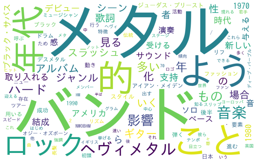
#@title Word Cloud with TF-IDF（All DATA)：🔲型 → #maskの#外すと🍩型に
# TF-IDF計算
tfidf_vec2 = vectorizer.fit_transform(df_all).toarray()[0]
# TF-IDFを辞書化
tfidf_dict2 = dict(zip(vectorizer.get_feature_names(), tfidf_vec2))
# 値が正のkeyだけ残す
tfidf_dict2 = {k: v for k, v in tfidf_dict2.items() if v > 0}

#Word Cloudで画像生成（#max_words, width, heightは任意設定）
wordcloud = WordCloud(background_color='white',
                      max_words=125,
                      #mask=custom_mask,
                      font_path='/usr/share/fonts/truetype/fonts-japanese-gothic.ttf',
                      width=1000,
                      height=600,
                      ).generate_from_frequencies(tfidf_dict2)

#生成した画像の表示
plt.figure(figsize=(15,10))
plt.imshow(wordcloud)
plt.axis("off")
plt.show()

※アンケート結果によるものではありませんが、以下出力イメージ例です。

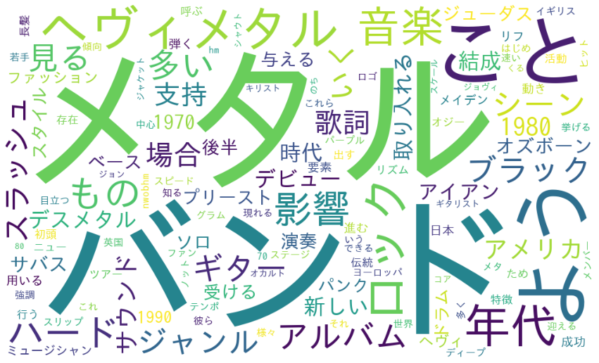
#@title Word Cloud with High CS Data (TF-IDF)：🔲型 → #maskの#外すと🍩型に
tfidf_vec = vectorizer.fit_transform(df_all_high_words).toarray()[0]
# TF-IDFを辞書化
tfidf_dict = dict(zip(vectorizer.get_feature_names(), tfidf_vec))
# 値が正のkeyだけ残す
tfidf_dict = {k: v for k, v in tfidf_dict.items() if v > 0}

#Word Cloudで画像生成（#max_words, width, heightは任意設定）
wordcloud = WordCloud(background_color='white',
                      max_words=125,
                      #mask=custom_mask,
                      font_path='/usr/share/fonts/truetype/fonts-japanese-gothic.ttf',
                      width=1000,
                      height=600,
                      ).generate_from_frequencies(tfidf_dict)

#生成した画像の表示
plt.figure(figsize=(15,10))
plt.imshow(wordcloud)
plt.axis("off")
plt.show()

#@title Word Cloud with Low CS Data (TF-IDF)：🔲型 → #maskの#外すと🍩型に
tfidf_vec = vectorizer.fit_transform(df_all_low_words).toarray()[0]
# TF-IDFを辞書化
tfidf_dict = dict(zip(vectorizer.get_feature_names(), tfidf_vec))
# 値が正のkeyだけ残す
tfidf_dict = {k: v for k, v in tfidf_dict.items() if v > 0}

#Word Cloudで画像生成（#max_words, width, heightは任意設定）
wordcloud = WordCloud(background_color='white',
                      max_words=125,
                      #mask=custom_mask,
                      font_path='/usr/share/fonts/truetype/fonts-japanese-gothic.ttf',
                      width=1000,
                      height=600,
                      ).generate_from_frequencies(tfidf_dict)

#生成した画像の表示
plt.figure(figsize=(15,10))
plt.imshow(wordcloud)
plt.axis("off")
plt.show()

**Userの訴えかけを語彙でグループ分け

クラスタリング（k-means法）について\
数値化（TF-IDF）した各意見のクラスタリングを行います。クラスタリングは、scikit-learn の KMeans（非階層的クラスタ分析）を使用します。KMeans（非階層的クラスタリング）では、設定したクラスタ数にしたがって、近い属性のデータをグループ化します。\
参考として適性なクラスター数を導く手法（エルボー法）の結果を表示します。横軸：クラスタ数、縦軸：SSE（残差平方和）としたグラフで、クラスタ数を増やしてもSSEがほとんど改善しない点のクラスタ数を選ぶというものです。\
適切な点が見いだせない場合も含め、クラスター数は任意に設定できるようにしています。「クラスター数設定」で設定します。

#@title **Option**：エルボー法（SSE値の低下がサチる場所を最適なクラスター数とみなす方法）

#ライブラリインポート
from sklearn.preprocessing import StandardScaler
from sklearn import preprocessing
from sklearn.cluster import KMeans

X=df_tfidf
sc = preprocessing.StandardScaler()
sc.fit(X)
X_norm = sc.transform(X)
#print(type(X_norm))

distortions = []

for i  in range(1,31):                # 1～30クラスタまで一気に計算 
    km = KMeans(n_clusters=i,
                init='k-means++',     # k-means++法によりクラスタ中心を選択
                n_init=10,
                max_iter=300,
                random_state=0)
    km.fit(X)                         # クラスタリングの計算を実行
    distortions.append(km.inertia_)   # km.fitするとkm.inertia_が得られる

plt.plot(range(1,31),distortions,marker='o')
plt.xlabel('Number of clusters')
plt.ylabel('Distortion')
plt.show()

#@title クラスター数設定 { run: "auto" }
num_clusters = 8 #@param {type:"number"}

#@title TF-IDF_k-meansによる各意見のクラス分け
# kmean_clustring
from sklearn.cluster import KMeans

# クラスタ数8で実行
clusters = KMeans(n_clusters=num_clusters).fit_predict(tfidf)

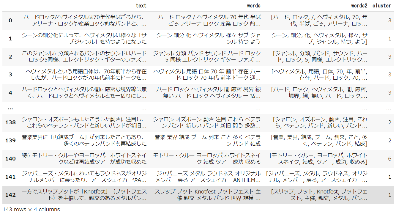
#データフレームにclusterを反映
df['cluster'] = clusters
df

※アンケート結果によるものではありませんが、以下出力イメージ例です。

最後に

アンケート分析で苦労するのは、「自由記述」など、自然言語です。
量がおおいと、ただただ圧倒されます。

まずは、全体をWord Cloudで眺めたり、満足度別に描いて眺めたりして、Userの訴えの全体感に思いを巡らせ、
その上で、語彙でグループ分け（クラスタ分け）した単位でUserの声に触れることで、より我がごととして染み込んできやすくなるように思います。
　
Pythonやその他ツールは分析の手助けはしてくれますが、答えを教えてくれるものではありません。
ダイレクトに答えは得られないまでも、できるだけ先の答えにつなげやすいであろう見方やまとめ方はできると思いますし、これらによって答えに近づくことができるのだと思います
。

参考サイト