2021/11/13:本文抽出+ノイズ除去済の「学問ノススメ」 ← 必要な方はこちらをクリック
はじめに
前回の記事では「TF-IDF」によるワードクラウド描画にチャレンジしましたが、思い通りにならなかった点(以下)がありましたので、再度チャレンジしました。
- scikit-learnの「TfidfVectorizer」というライブラリがうまく使えなかった…
- nlplot(自然言語可視化・分析ライブラリ)もフルで試せなかった
実力不足のため、苦労しましたが、なんとか任意のテキストデータで「Word Cloud」、「nlplotによる各種可視化」、「(TfidfVectorizer)によるTF-IDF計算」、「TF-IDFによるWord Cloud」が実行できるようになったたので、備忘も兼ね、記事にしたものです。
実行条件など
・Google colabで実行
・**青空文庫の「学問ノススメ」**で実行
※コードは任意データでの実行を意図していますので、「こころ」限定ではありません。
備忘
- 読み込ませたテキストデータは、見やすさ・扱いやすさからデータフレームにした。
- 分かち書きは、スペース区切り(語A 語B 語C)とカンマ区切り [語A,語B,語C] の2パターンとした。1パターンだけで対応したかったが…私の修行が足りないのであろう。TF-IDF計算はスペース区切り、Word Cloudは カンマ区切り、nlplotはどちらでもいけたと思う。
- 文章は「。」でセンテンスに分けた。TF-IDFの計算・TF-IDFによるWord Cloud描画は、センテンス毎と全文書の2通りとした。
- 品詞は一般名詞・動詞・形容詞(動詞と形容詞は基礎型)を対象とした。
ライブラリのインストール
# nlplotをインストール
pip install nlplot
# 日本語フォントをインストール
!apt-get -y install fonts-ipafont-gothic
# Mecabのインストール
!pip install mecab-python3==0.996.5
from pathlib import Path
import pandas as pd
import MeCab
import matplotlib.pyplot as plt
テキストファイル & ストップワード指定
# テキストファイル名を指定(※textファイルの文字コードは「UTF-8」としてください)
filename = 'sample.txt'
# ストップワード設定
stop_words = ["し","い","ある", "おる", "せる", "ない", "いる", "する", "の", "よう", "なる", "それ", "そこ", "これ", "こう", "ため", "そう", "れる", "られる"]
モジュールの準備
- 前処理(改行や空白の処理、センテンス化)や形態素分析、ワード出現回数処理を行います。
- 文章をワードに分解後、一般名詞・動詞・形容詞(動詞と形容詞は基礎型)のみを取り出しています。(※追加や変更はコード操作が必要です)
import MeCab as mc
import re           # 正規表現
import numpy as np
with open(filename, 'r', encoding='utf-8') as file:
    lines = file.readlines()

# with open(filename, 'r', encoding='utf-8') as all:
#    all_text = all.readlines()

source = open(filename, 'r', encoding='utf-8')
all_text = source.read()
all_text = ''.join(all_text)
table = str.maketrans({
  '\u3000': '',
  ' ': '',
  '\t': ''
})
all_text = all_text.translate(table)

lines = [l.strip() for l in lines]
all_text = [l.strip() for l in all_text]

sentences = []
for sentence in lines:
    texts = sentence.split('。')
    sentences.extend(texts)
all_text = ''.join(all_text)
all_text
# 抽出したワードをデータフレームdfに
import pandas as pd
import numpy as np
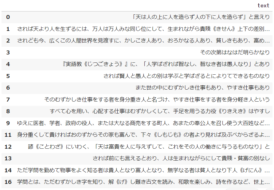
df_text = pd.DataFrame(sentences, columns = ['text'], index=None)
# 空白をNaNに置き換え
df_text['text'].replace('', np.nan, inplace=True)
# Nanを削除 inplace=Trueでdf上書き
df_text.dropna(subset=['text'], inplace=True)
df_text[:15]
# スペース区切り分かち書き
def mecab_analysis(text):
t = MeCab.Tagger('-Ochasen')
node = t.parseToNode(text)
words = []
while node:
if node.surface != "": # ヘッダとフッタを除外
word_type = node.feature.split(',')[0]
sub_type = node.feature.split(',')[1]
features_ = node.feature.split(',')
#品詞を選択
if word_type in ["名詞"]:
if sub_type in ['一般']:
word = node.surface
words.append(word)
#動詞、形容詞[基礎型]を抽出(名詞のみを抽出したい場合は以下コードを除く)
elif word_type in ['動詞','形容詞'] and not (features_[6] in stop_words):
words.append(features_[6])
node = node.next
if node is None:
break
return " ".join(words)
# カンマ区切り分かち書き
def mecab_analysis2(text):
t = MeCab.Tagger('-Ochasen')
node = t.parseToNode(text)
words2 = []
while(node):
if node.surface != "": # ヘッダとフッタを除外
word_type = node.feature.split(',')[0]
sub_type = node.feature.split(',')[1]
features_ = node.feature.split(',')
if word_type in ['名詞']: # 名詞をリストに追加する
if sub_type in ['一般']:
words2.append(node.surface)
#動詞、形容詞[基礎型]を抽出(名詞のみを抽出したい場合は以下コードを除く)
elif word_type in ['動詞','形容詞'] and not (features_[6] in stop_words):
words2.append(features_[6])
node = node.next
if node is None:
break
return words2
# スペース区切り分かち書き(全文書一括)
def mecab_analysis3(text):
t = MeCab.Tagger('-Ochasen')
node = t.parseToNode(all_text)
words3 = []
while node:
if node.surface != "": # ヘッダとフッタを除外
word_type = node.feature.split(',')[0]
sub_type = node.feature.split(',')[1]
features_ = node.feature.split(',')
#品詞を選択
if word_type in ["名詞"]:
if sub_type in ['一般']:
all_text_word = node.surface
words3.append(all_text_word)
#動詞、形容詞[基礎型]を抽出(名詞のみを抽出したい場合は以下コードを除く)
elif word_type in ['動詞','形容詞'] and not (features_[6] in stop_words):
words3.append(features_[6])
node = node.next
if node is None:
break
return " ".join(words3)
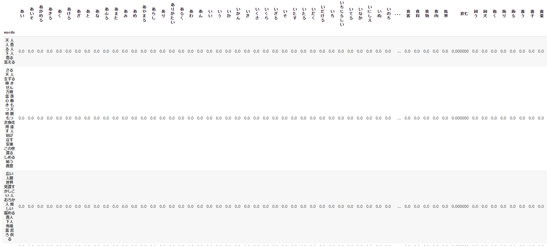
# 形態素結果をリスト化し、データフレームdfに結果を列追加する
df_text['words'] = df_text['text'].apply(mecab_analysis)
df_text['words2'] = df_text['text'].apply(mecab_analysis2)
df_text[:15]
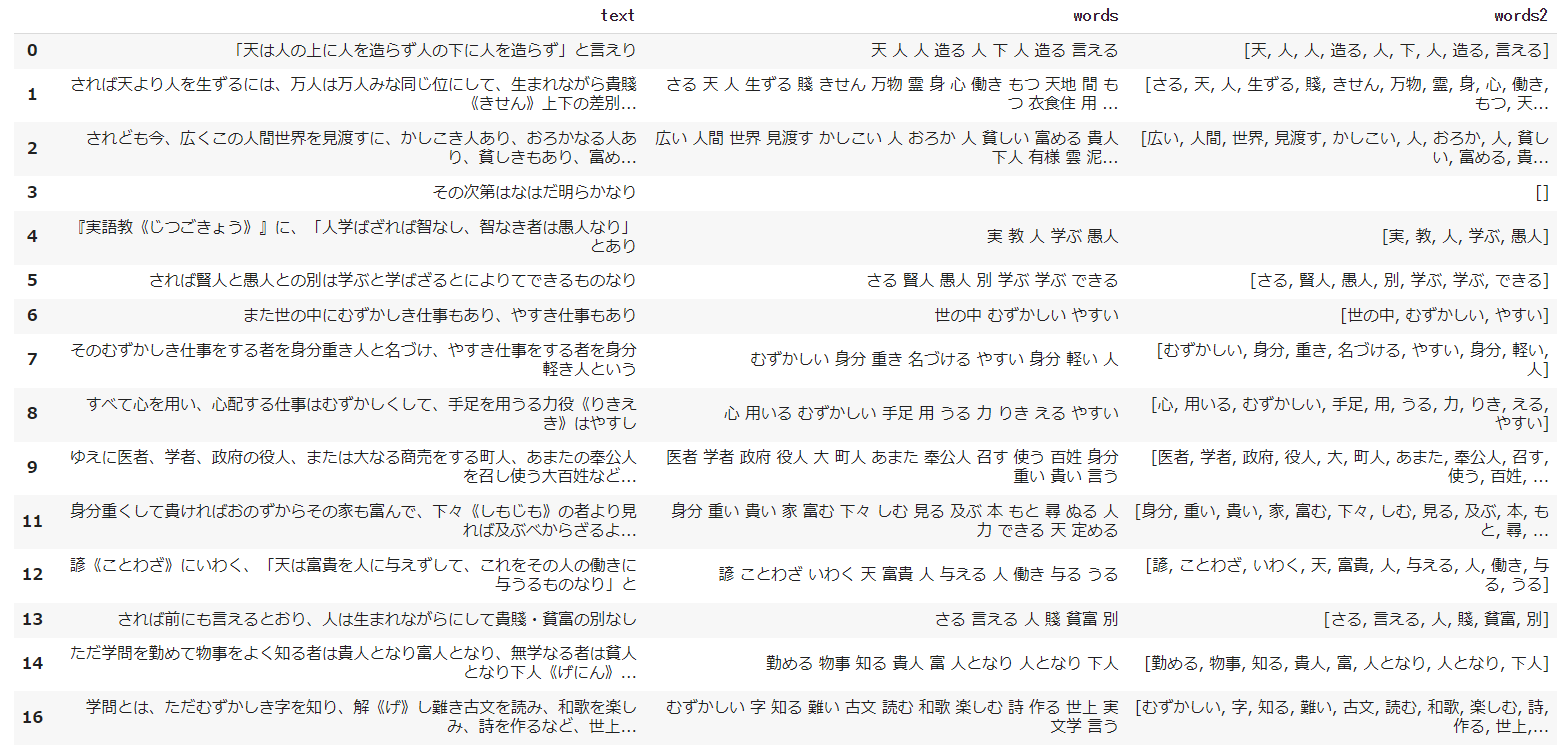
この表を見ると、各センテンスからの語の抽出状況がよくわかります。
textがセンテンス、wordsがスペース区切り分かち書き、words2がカンマ区切り分かち書きが格納されています。
df = pd.Series(all_text)
df = df.apply(mecab_analysis3)
# filter the df to one candidate, and create a list of responses from them
words_list = df_text.words2.tolist()
words_list = sum(words_list,[])

from collections import Counter

# 出現回数を集計し、最頻順にソート
words_count = Counter(words_list)
result = words_count.most_common()

# 出現回数結果の画面出力
for word, cnt in result:
    print(word, cnt)
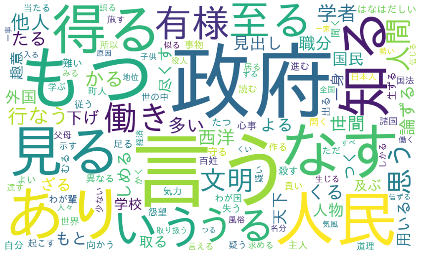
ワードクラウド
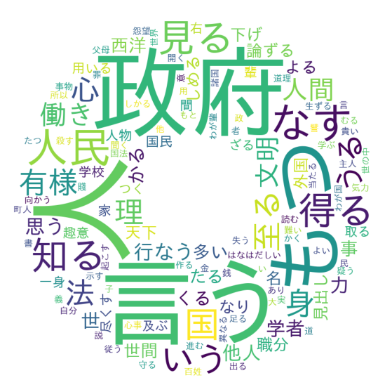
- ワードクラウドは、文章中で出現頻度が高い単語を複数選び出し、その頻度に応じた大きさで図示する手法です。
- ワードクラウドは任意の形状に描画できるため、以下では①長方形(通常)と②ドーナツ型の2パターンで示しています。
ワードクラウド
# wordcloud取込用に辞書型ヘ変換
dic_result = dict(result)

# Word Cloudで画像生成
from wordcloud import WordCloud

wordcloud = WordCloud(background_color='white',
                      max_words=125,
                      font_path='/usr/share/fonts/truetype/fonts-japanese-gothic.ttf',
                      width=1000,
                      height=600,
                      ).fit_words(dic_result)

# 生成した画像の表示
import matplotlib.pyplot as plt
from matplotlib import rcParams

plt.figure(figsize=(15,10))
plt.imshow(wordcloud)
plt.axis("off")
plt.show()

ワードクラウド描画(ドーナツ型)
# donutsデータダウンロード
import requests

url = "https://github.com/hima2b4/Word-Cloud/raw/main/donuts.png"
# url = "https://github.com/hima2b4/Word-Cloud/raw/main/biwa.png"

file_name = "donuts.png"
# file_name = "biwa.png"

response = requests.get(url)
image = response.content

with open(file_name, "wb") as f:
    f.write(image)
# ライブラリインポート
from PIL import Image
import numpy as np

custom_mask = np.array(Image.open('donuts.png'))
wordcloud = WordCloud(background_color='white',
                      max_words=125,
                      mask=custom_mask,
                      font_path='/usr/share/fonts/truetype/fonts-japanese-gothic.ttf',
                      width=1200,
                      height=1200
                      ).fit_words(dic_result)

# 生成した画像の表示
plt.figure(figsize=(15,10))
plt.imshow(wordcloud)
plt.axis("off")
plt.show()
nlplot
「nlplot」は、自然言語の可視化・分析できるライブラリです。
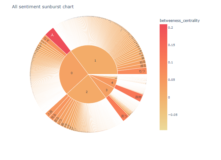
- N-gram bar chart, N-gram tree Map, Histogram of the word count, wordcloud, co-occurrence networks(共起ネットワーク), sunburst chart(サンバースト)を描きます。
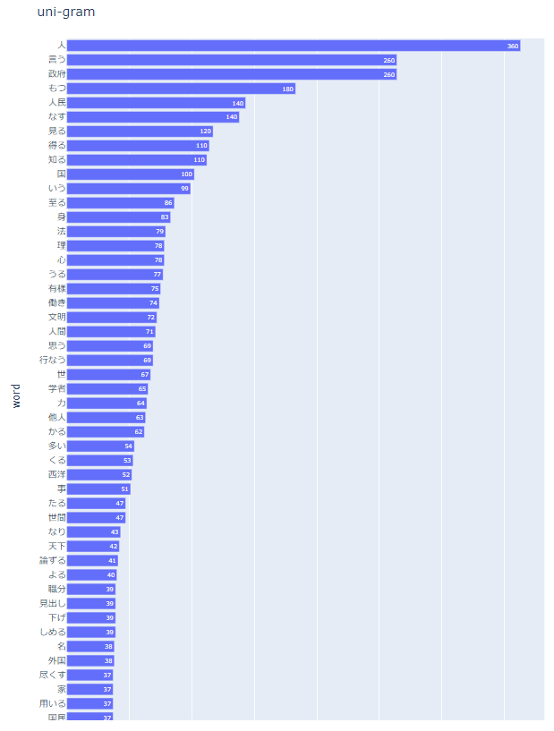
nlplot(uni-gram)
import nlplot

npt = nlplot.NLPlot(df_text, target_col='words')

# top_nで頻出上位単語, min_freqで頻出下位単語を指定できる
# stopwords = npt.get_stopword(top_n=0, min_freq=0)  #前処置にて除去しているため適用していない

npt.bar_ngram(
    title='uni-gram',
    xaxis_label='word_count',
    yaxis_label='word',
    ngram=1,
    top_n=50,
#    stopwords=stopwords,
)
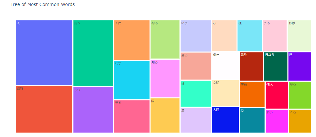
nlplot(tree-map)
npt.treemap(
    title='Tree of Most Common Words',
    ngram=1,
    top_n=30,
#    stopwords=stopwords,  #前処置にて除去しているため適用していない
)
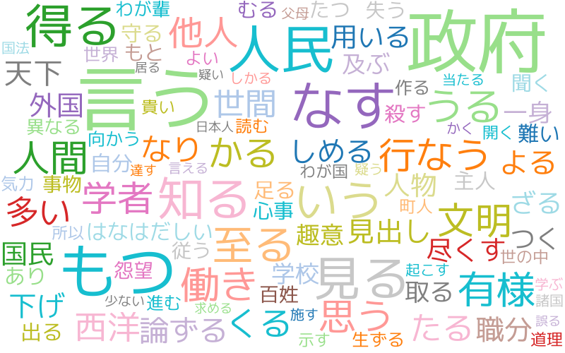
nlplot(wordcloud)
npt.wordcloud(
    max_words=100,
    max_font_size=100,
    colormap='tab20_r',
#    stopwords=stopwords,  #前処置にて除去しているため適用していない
)
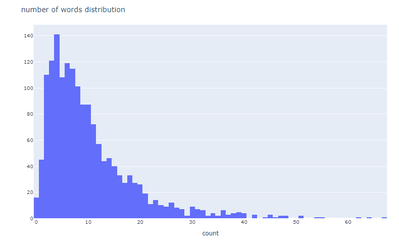
nlplot(word_distribution)
# 単語数の分布
npt.word_distribution(
    title='number of words distribution',
    xaxis_label='count',
)
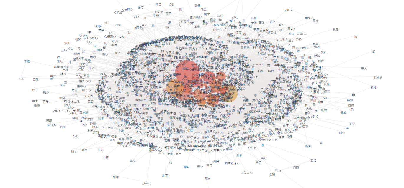
nlplot(build_graph)
# ビルド(データ件数によっては処理に時間を要します)※ノードの数のみ変更
npt.build_graph(min_edge_frequency=1,
                #stopwords=stopwords,
                )

display(
    npt.node_df.head(), npt.node_df.shape,
    npt.edge_df.head(), npt.edge_df.shape
)

npt.co_network(
    title='Co-occurrence network',
)
nlplot(sunburst)
npt.sunburst(
    title='All sentiment sunburst chart',
    colorscale=True,
    color_continuous_scale='Oryel',
    width=800,
    height=600,
    #save=True
)
TF-IDF
TF-IDF は ワードの重要度 を測るための指標の1つ。ワードの出現頻度とレア度が考慮された指標。TF、IDF、TF-IDF の定義は以下の通り。
\begin{eqnarray} TF(d,w) &=& \frac{文書d における語wの出現回数}{文書d における全語の出現回数の和}\ IDF(w) &=& log(\frac{全文書数}{語w を含む文書数})\ TFIDF(d,w) &=& TF(d,w) \times IDF(w) \end{eqnarray}
- sentence毎にTF-IDFを算出、sentence×wordマトリクスをcsv出力(tfidf.csv)します。
- [参考] 指定したsentenceのWord cloudを描きます。※sentenceは個別指定
- 文書全体でTF-IDFを算出した時のWord cloudも描きます。
from sklearn.feature_extraction.text import TfidfVectorizer

# TF-IDFをデータフレームに展開(センテンス×word)
vectorizer = TfidfVectorizer(use_idf=True)
tfidf = vectorizer.fit_transform(df_text['words'])

df_tfidf = pd.DataFrame(tfidf.toarray(), columns=vectorizer.get_feature_names(), index=df_text['words'])
display(df_tfidf)
# sentence×TF-IDFをcsv形式で出力
from google.colab import files
df_tfidf.to_csv('tfidf.csv',encoding='utf_8_sig')
# files.download('tfidf.csv')
[参考サイト]
Word Cloud with TF-IDF for each Sentence
指定したsentenceのWord Cloudを表示しているだけなので参考程度。
※tfidf_vec = vectorizer.fit_transform(df_text['words']).toarray()[0] ←この数値で描画したいsentenceを指定する。
tfidf_vec = vectorizer.fit_transform(df_text['words']).toarray()[0]
# 単語: tf-idfの辞書にする。
tfidf_dict = dict(zip(vectorizer.get_feature_names(), tfidf_vec))
# 値が正のkeyだけ残す
tfidf_dict = {k: v for k, v in tfidf_dict.items() if v > 0}
# Word Cloudで画像生成
wordcloud = WordCloud(background_color='white',
                      max_words=125,
                      font_path='/usr/share/fonts/truetype/fonts-japanese-gothic.ttf',
                      width=1000,
                      height=600,
                      ).generate_from_frequencies(tfidf_dict)

# 生成した画像の表示
plt.figure(figsize=(15,10))
plt.imshow(wordcloud)
plt.axis("off")
plt.show()

Word cloud with TF-IDF for All texts
tfidf_vec2 = vectorizer.fit_transform(df).toarray()[0]
# 単語: tf-idfの辞書にする。
tfidf_dict2 = dict(zip(vectorizer.get_feature_names(), tfidf_vec2))
# 値が正のkeyだけ残す
tfidf_dict2 = {k: v for k, v in tfidf_dict2.items() if v > 0}
# Word Cloudで画像生成
wordcloud = WordCloud(background_color='white',
                      max_words=125,
                      font_path='/usr/share/fonts/truetype/fonts-japanese-gothic.ttf',
                      width=1000,
                      height=600,
                      ).generate_from_frequencies(tfidf_dict2)

# 生成した画像の表示
plt.figure(figsize=(15,10))
plt.imshow(wordcloud)
plt.axis("off")
plt.show()
最後に
すこし冗長的なコードもあると思いますが、なんとかやりたいことはできました。
nlplot含め、使用したライブラリは本当にすばらしいです。
テキストから何かを探りたい、何か探れないか?でもいいと思います。
ぜひ実行いただければと思います。
最後まで見ていただきありがとうございました。
参考サイト