随時更新する予定
最初のおまじない
図を閉じ,データを初期化し,コンソールウィンドウを綺麗にします.
%% Start of script

close all;                          % close all figures
clear;                              % clear all variables
clc;                                % clear the command terminal
データをコマンドウィンドウに表示する
セミコロンをつけないだけでも可視化はできるが,disp 関数を使うと丁寧.
foo = 'Hello world!';
disp(foo);

hoge = 1:10;
disp(hoge);

data = rand(3,3);
disp(data);
結果
Hello world!
     1     2     3     4     5     6     7     8     9    10

    0.7922    0.0357    0.6787
    0.9595    0.8491    0.7577
    0.6557    0.9340    0.7431
連続した値を出力する
いくつか手法がある.コロン演算子と linspace は挙動が似ている.lispace はデフォルトで入力範囲を100分割する.
-5:5

-5:0.1:5

linspace(-5,5)
グラフを描画する
plot を使います.時系列の場合には第一引数に time, 第二引数に data を入れます.
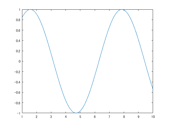
time = 1:0.1:10;
data = sin(time);

plot(time, data);
現在の図やグラフのハンドルを取得する
MATLAB のハンドルとは参照やポインタのようなものです.gcf や gca という機能を使うことができます.MATLAB のリファレンス等によく出てくるので覚えたほうが良いでしょう.ちなみに gcf は "Get Current Figure" の略で,gca は "Get Current Axis" の略です.Figure は図全体を示すのに対して,Axis はグラフを示します.
time = 1:0.1:10;
data = sin(time);

plot(time, data);

disp(gcf);
disp(gca);
結果
  Figure (1) のプロパティ:

      Number: 1
        Name: ''
       Color: [0.9400 0.9400 0.9400]
    Position: [360 502 560 420]
       Units: 'pixels'

  get を使用してすべてのプロパティを表示

  Axes のプロパティ:

             XLim: [1 10]
             YLim: [-1 1]
           XScale: 'linear'
           YScale: 'linear'
    GridLineStyle: '-'
         Position: [0.1300 0.1100 0.7750 0.8150]
            Units: 'normalized'

  get を使用してすべてのプロパティを表示
フォントを変更する
set 関数がよく使われます.gca と組み合わせると使いやすいでしょう.
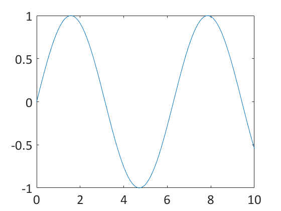
time = 0:0.1:10;
data = sin(time);

plot(time, data);

set(gca,'FontName','Calibri','FontSize',20);
テキストを読み込む
fileID = fopen('test.txt','r');
fileData = textscan(fileID, '%s','Delimiter','\n');
fclose(fileID);
読み込んだテキストの行数だけループを回す
fileID = fopen('test.txt','r');
fileData = textscan(fileID, '%s','Delimiter','\n');
fclose(fileID);

graphList = fileData{1};
graphListLength = length(graphList);

for index = 1:graphListLength
    disp(index);
end
文字列を接続する
strcat と strjoin がある.最近は strjoin がお気に入り.
fileID = fopen('test.txt','r');
fileData = textscan(fileID, '%s','Delimiter','\n');
fclose(fileID);

graphList = fileData{1};
graphListLength = length(graphList);

for index = 1:graphListLength
    dataName = graphList{index};
    dataNameWithExtention = strjoin({dataName, 'csv'}, '.');
end
数値を文字列に変換する
num2str を使う.
number = 1.11;
name = num2str(number);
disp(name);
文字列を置換する
strrep を使う.小数などを文字列に変換した際,拡張子のドットと小数点が混ざり都合が悪いときがある.
number = 1.11;
name = num2str(number);
disp(name);

replacedName = strrep(name, '.', '_');
disp(replacedName);
組み合わせると読みづらいが短くなる
number = 1.11;
name = num2str(number);
disp(name);

replacedName = strrep(name, '.', '_');
disp(replacedName);

combinedName = strjoin({strrep(num2str(number),'.', '_'),'emf'}, '.');
disp(combinedName);
CSVを読み込む
readtable を最近使っています.csvread は文字列に弱いのでおすすめしません.
graphData = readtable('timeSeriesData.csv');
time = graphData{:,1};
CSVを出力する
writetable csvwrite dlmwrite あります.こっちは逆に csvwrite をよく使ってます.書式を詳しく設定したい場合には dlmwrite が便利です.
t = 0:pi/50:10*pi;
st = sin(t);
ct = cos(t);

figure
plot3(st,ct,t)

data = [st', ct', t'];
csvwrite('trajectory.csv', data);
dlmwrite('trajectory.txt', data, 'delimiter', ',', 'newline', 'pc', 'precision', '%10.5f');
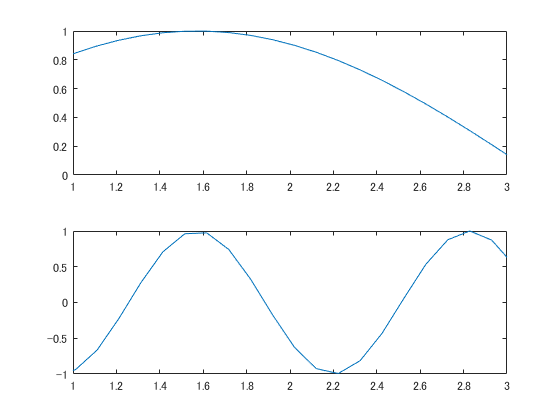
上下に並べてグラフを出力する
subplotを用いる.
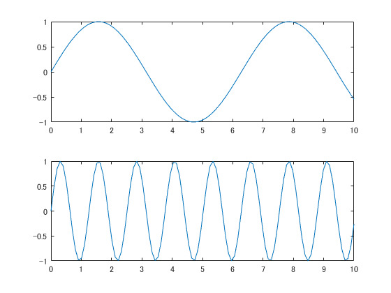
x = linspace(0,10);
y1 = sin(x);
y2 = sin(5*x);

figure
subplot(2,1,1);
plot(x,y1)

subplot(2,1,2);
plot(x,y2)
グラフの軸を同期させる
linkaxesを使う.図を詳しく見る場合に役に立ちます.
x = linspace(0,10);
y1 = sin(x);
y2 = sin(5*x);

figure
ax1 = subplot(2,1,1);
plot(x,y1)

ax2 = subplot(2,1,2);
plot(x,y2)

linkaxes([ax1,ax2],'x')
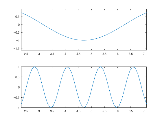
軸の範囲を決める
xlim等が使えます.
x = linspace(0,10);
y1 = sin(x);
y2 = sin(5*x);

figure
ax1 = subplot(2,1,1);
plot(x,y1)

ax2 = subplot(2,1,2);
plot(x,y2)

linkaxes([ax1,ax2],'x')

xlim([1 3])
図を保存する
figure を画像に保存します.fig ファイルで保存してもいいけど,powerpoint 等に貼り付ける場合には emf がおすすめ.
x = linspace(0,10);
y1 = sin(x);
y2 = sin(5*x);

figure
ax1 = subplot(2,1,1);
plot(x,y1)

ax2 = subplot(2,1,2);
plot(x,y2)

linkaxes([ax1,ax2],'x')

xlim([1 3])

saveas(gcf,'image','emf');
図に文字を載せる
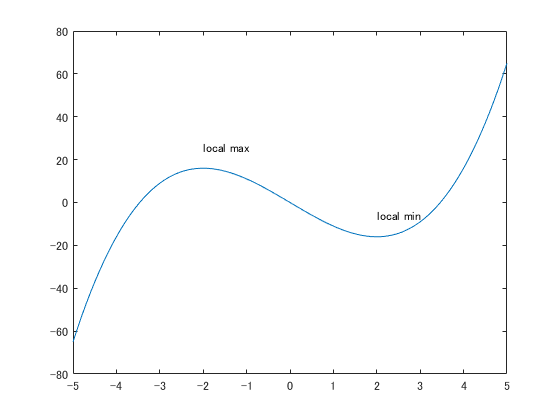
x = linspace(-5,5);
y = x.^3-12*x;
plot(x,y)

xt = [-2 2];
yt = [16 -16];
str = {'local max','local min'};
text(xt,yt + 10,str)
グリッド・ラベル・タイトルを表示する
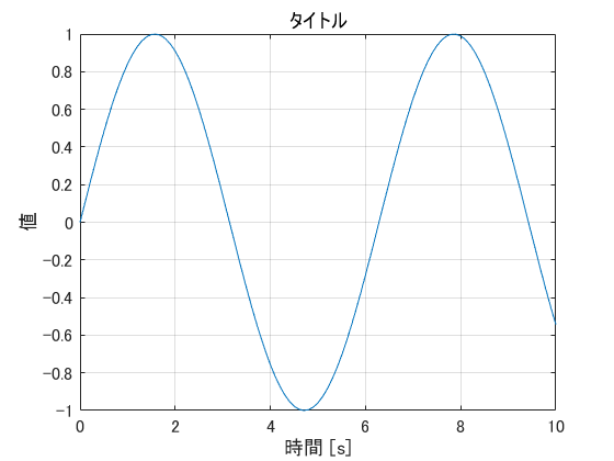
time = 0:0.1:10;
data = sin(time);

figure;
plot(time, data);
xlabel('時間 [s]');
ylabel('値');
title('タイトル');

box on;
grid on;
set(gca,'FontSize',12);
ピークを検出する
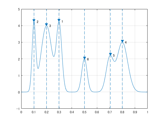
x = linspace(0,1,1000);

Pos = [1 2 3 5 7 8]/10;
Hgt = [4 4 4 2 2 3];
Wdt = [2 6 3 3 4 6]/100;

for n = 1:length(Pos)
    Gauss(n,:) =  Hgt(n)*exp(-((x - Pos(n))/Wdt(n)).^2);
end

PeakSig = sum(Gauss);
plot(x,Gauss,'--',x,PeakSig);
[psor,lsor] = findpeaks(PeakSig,x,'SortStr','descend');
findpeaks(PeakSig,x)
text(lsor+.02,psor,num2str((1:numel(psor))'))

for i = 1:length(lsor)
    x = lsor(i);
    line([x, x], ylim, 'LineStyle','--');
end
データの補間を行う
interp1 が便利
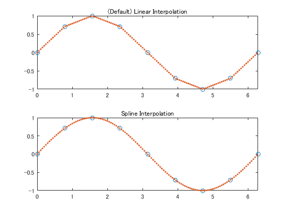
x = 0:pi/4:2*pi;
v = sin(x);
xq = 0:0.05:2*pi; %適当な数

subplot(2,1,1);
vq1 = interp1(x,v,xq);
plot(x,v,'o',xq,vq1,':.');
xlim([0 2*pi]);
title('(Default) Linear Interpolation');

subplot(2,1,2);
vq2 = interp1(x,v,xq,'spline');
plot(x,v,'o',xq,vq2,':.');
xlim([0 2*pi]);
title('Spline Interpolation');
ローパスフィルタをかける
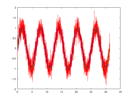
time = 0:0.01:pi*10;
correctData = sin(time)';
noisyData = sin(time)' + 0.25 * randn(length(time),1);

low = 10;
[B,A] = butter(3,2*low/length(noisyData), 'low');
filteredData = filtfilt(B,A,noisyData);

plot(time, noisyData,'r');
hold on;

plot(time, correctData, 'g');
plot(time, filteredData, 'b');
hold off;
外れ値を削除する
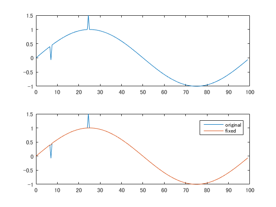
time = 0:0.5:99;
x = sin(2*pi*time/100);
x(15) = x(15) - 0.5;
x(50) = x(50) + 0.5;

xFixed = hampel(x);

subplot(2,1,1);
plot(time, x);

subplot(2,1,2);
plot(time, x, time, xFixed);
legend('original', 'fixed');
動画を書き出す
videowriter を使います
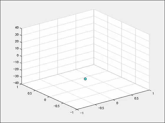
z = -10*pi:pi/25:10*pi;
x = (cos(2*z).^2).*sin(z);
y = (sin(2*z).^2).*cos(z);

tx = x(1);
ty = y(1);
tz = z(1);

writerObj = VideoWriter('test.mp4', 'MPEG-4');
open(writerObj);

fig = scatter3(tx, ty, tz,'MarkerEdgeColor','k',...
        'MarkerFaceColor',[0 1.0 1.0]);
set(fig, 'XDataSource', 'tx');
set(fig, 'YDataSource', 'ty');
set(fig, 'ZDataSource', 'tz');
set(gca, 'Xlim', [-1 1], 'Ylim', [-1 1], 'Zlim', [-40 40]);
set(gca,'nextplot','replacechildren');

for k = 1:length(z)
    tx = x(k);
    ty = y(k);
    tz = z(k);

    refreshdata(fig);
    frame = getframe(gcf);
    writeVideo(writerObj, frame);
end

close(writerObj);
常微分方程式を解く
ode45が便利.ラムダ式を使うこともできる.
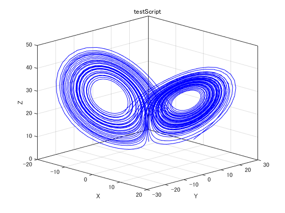
function dx = lorenz(t, x)

% Standard constants for the Lorenz Attractor
sigma = 10;
rho = 28;
beta = 8/3;

% I like to initialize my arrays
dx = [0; 0; 0];

% The lorenz strange attractor
dx(1) = sigma*(x(2)-x(1));
dx(2) = x(1)*(rho-x(3))-x(2);
dx(3) = x(1)*x(2)-beta*x(3);
odeFunction = @(t, x)(lorenz(t, x));

maxTime = 60;
[t, y] = ode45(odeFunction, [0 maxTime], [10 10 10]);

titleString = 'testScript';
figure1Title = strcat('XYZ 3DPlot', titleString);
figure1 = figure('Name', figure1Title);
axes1 = axes('Parent',figure1);
hold on;
plot3(y(:,1), y(:,2), y(:,3),'Color',[0 0 1]);
title(titleString);
xlabel('X');
ylabel('Y');
zlabel('Z');
view(axes1,[45.3 20.4]);
grid on;
box on;
hold off;