python3で自己相関関数

久々に読んだら，規格化数列がまどろっこしかったので修正し実行速度を再測定．
マシンが変わったので実行速度も変化した．

---

久々に読んだら関数名が意味不明だったので比較した関数の説明を追記．

---

なんか，思った通りの結果が出なかったので計算内容を確認したのと実行速度を測定したのと．

比較した関数

• corr1
  • hadacchi の自作関数
  • numpyのベクトル演算でlagだけずらした時系列間の積をとり，その積のベクトルをmeanメソッドで平均して自己相関を計算する関数
  • 他の3関数と比較して周期関数のピークが減衰せずに出てくる（正弦波の自己相関関数が減衰するとか明らかにおかしい）というメリットはありつつも， デメリットとしてnlagsをあまりに大きい値にしてしまうと，相関を計算するサンプルが少なすぎて相関係数の値が不安定（時系列をサンプルする毎に大きく値が変化してしまう）になる点がある
• corr3
  • corr2は作ったけど意味なかったので消して欠番
  • numpyのベクトル演算までは一緒だがsumメソッドで内積を計算した後，原系列長で除算して平均して自己相関を計算する関数
    • lagだけ時系列をシフトするとリテラル数が減るのに除算の母数が原系列長と一定なので変だと思うんだけど，この関数と比較することで，実はscipyとかstatsmodelsなんかの自己相関関数はこの実装になっていることに気付いた
• statsmodels.api.tsa.acf
  • statsmodelsモジュールにある自己相関関数を計算してくれる関数
  • いかなるlagの相関係数の計算であっても原系列長で除算していることが，corr3との比較で分かった
• scipy.signal.correlate
  • scipyモジュールにある自己相関関数を計算してくれる関数…かと思いきや内積しか計算してくれないから，ユーザが返り値を原系列長とかで除算しないと使えない

検算

コード

import scipy.signal as sig
import numpy as np
import statsmodels.api as sm
import matplotlib.pyplot as plt
import pandas
from IPython.core.display import display

x = np.arange(0,10000,0.1)
y = np.sin(x)
ny = (y-y.mean())/y.std()
dfy = pandas.DataFrame({'y':y})

def corr1(ts1, ts2, nlags=40):
    ts1, ts2 = np.asarray(ts1), np.asarray(ts2)
    nlags += 1
    N      = min(len(ts1),len(ts2))
    nts1   = ((ts1-ts1.mean())/ts1.std())[:N]
    nts2   = ((ts2-ts2.mean())/ts2.std())[:N]
    nlags  = min(N,nlags)
    result = [(nts1*nts2).mean()]
    for lag in range(1,nlags):
        result.append((nts1[lag:]*nts2[:-lag]).mean())
    return np.asarray(result)

def corr3(ts1, ts2, nlags=40):
    ts1, ts2 = np.asarray(ts1), np.asarray(ts2)
    nlags += 1
    N      = min(len(ts1),len(ts2))
    nts1   = ((ts1-ts1.mean())/ts1.std())[:N]
    nts2   = ((ts2-ts2.mean())/ts2.std())[:N]
    nlags  = min(N,nlags)
    result = [(nts1*nts2).sum()/N]
    for lag in range(1,nlags):
        result.append((nts1[lag:]*nts2[:-lag]).sum()/N)
    return np.asarray(result)

acf = sm.tsa.acf(y, nlags=5000)
sigcorr_buf = sig.correlate(ny,ny,mode='same')
sigcorr = sigcorr_buf[len(sigcorr_buf)//2:]  # 負のlagは消す
sigcorr /= len(sigcorr_buf)  # 系列長で規格化

myacf1 = corr1(y,y,nlags=5000)
myacf3 = corr3(y,y,nlags=5000)

display(pandas.DataFrame({ 'acf':acf
                         , 'corr1':myacf1
                         , 'corr3':myacf3
                         , 'sigcorr/N':sigcorr[:5001]
                         }))

result

まとめると，

• statsmodels.api.tsa.acfはlagが1以上の場合も，0の場合と同じ系列長を母数として平均値を計算している
• scipy.signal.correlateはそもそも原信号の規格化すらしてないので，全部手でやる必要がある
• scipy.signal.correlateは負の方向のlagにも計算をするため前半の結果は捨てても良い
  • 実は自己相関もFFTも実数系列を対象に処理すると正負方向に線対称なので，ホントは計算量を半分くらいに削減できるはずである
  • バタフライ演算から直さないといけないので，詳しくは numerical recipes を見る
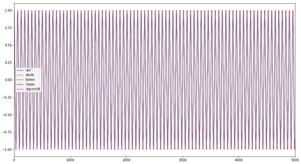
• 平均をちゃんと取るcorr1（mean）と比べて絶対値で少し小さくなるのは，lagが大きくなると，例えばlag=4000では コンボリュージョンの計算に 10000-4000=6000 個の値しか使えてないのに，平均値の計算をlags=10000で計算しているため
  • なので，正弦波の自己相関を計算した場合，画像のように前者は自己相関のピーク値が減衰していくが，corr1は減衰しない

idx	acf	corr3	corr1	sigcorr/N
0	1.000000	1.000000	1.000000	1.000000
1	0.996869	0.996869	0.996879	0.996869
2	0.987520	0.987520	0.987540	0.987520
3	0.972032	0.972032	0.972061	0.972032
4	0.950536	0.950536	0.950574	0.950536
5	0.923214	0.923214	0.923260	0.923214
6	0.890298	0.890298	0.890352	0.890298
7	0.852067	0.852067	0.852126	0.852067
8	0.808842	0.808842	0.808906	0.808842
9	0.760986	0.760986	0.761055	0.760986
10	0.708902	0.708902	0.708973	0.708902
11	0.653023	0.653023	0.653095	0.653023
12	0.593815	0.593815	0.593886	0.593815
13	0.531767	0.531767	0.531836	0.531767
14	0.467389	0.467389	0.467454	0.467389
15	0.401208	0.401208	0.401268	0.401208
16	0.333761	0.333761	0.333814	0.333761
17	0.265590	0.265590	0.265635	0.265590
18	0.197240	0.197240	0.197276	0.197240
19	0.129250	0.129250	0.129275	0.129250
20	0.062149	0.062149	0.062162	0.062149
21	-0.003546	-0.003546	-0.003547	-0.003546
22	-0.067341	-0.067341	-0.067356	-0.067341
23	-0.128762	-0.128762	-0.128791	-0.128762
24	-0.187364	-0.187364	-0.187409	-0.187364
25	-0.242735	-0.242735	-0.242796	-0.242735
26	-0.294497	-0.294497	-0.294574	-0.294497
27	-0.342314	-0.342314	-0.342406	-0.342314
28	-0.385888	-0.385888	-0.385996	-0.385888
29	-0.424967	-0.424967	-0.425091	-0.424967
...	...	...	...	...
4971	-0.089497	-0.089497	-0.094179	-0.089497
4972	-0.113837	-0.113837	-0.119793	-0.113837
4973	-0.140299	-0.140299	-0.147641	-0.140299
4974	-0.168542	-0.168542	-0.177364	-0.168542
4975	-0.198200	-0.198200	-0.208576	-0.198200
4976	-0.228886	-0.228886	-0.240871	-0.228886
4977	-0.260194	-0.260194	-0.273822	-0.260194
4978	-0.291705	-0.291705	-0.306987	-0.291705
4979	-0.322991	-0.322991	-0.339915	-0.322991
4980	-0.353620	-0.353620	-0.372153	-0.353620
4981	-0.383160	-0.383160	-0.403245	-0.383160
4982	-0.411182	-0.411182	-0.432741	-0.411182
4983	-0.437269	-0.437269	-0.460201	-0.437269
4984	-0.461016	-0.461016	-0.485199	-0.461016
4985	-0.482038	-0.482038	-0.507329	-0.482038
4986	-0.499972	-0.499972	-0.526208	-0.499972
4987	-0.514479	-0.514479	-0.541483	-0.514479
4988	-0.525255	-0.525255	-0.552830	-0.525255
4989	-0.532025	-0.532025	-0.559962	-0.532025
4990	-0.534555	-0.534555	-0.562631	-0.534555
4991	-0.532649	-0.532649	-0.560630	-0.532649
4992	-0.526151	-0.526151	-0.553797	-0.526151
4993	-0.514953	-0.514953	-0.542016	-0.514953
4994	-0.498989	-0.498989	-0.525219	-0.498989
4995	-0.478243	-0.478243	-0.503387	-0.478243
4996	-0.452743	-0.452743	-0.476551	-0.452743
4997	-0.422566	-0.422566	-0.444793	-0.422566
4998	-0.387838	-0.387838	-0.408242	-0.387838
4999	-0.348727	-0.348727	-0.367077	-0.348727
5000	-0.305450	-0.305450	-0.321526	-0.305450

プロット

速度測定

先に信号を100系列作っておいて，自己相関を計算する．

コード

import copy
import scipy.signal as sig
import numpy as np
import statsmodels.api as sm
import time
import matplotlib.pyplot as plt
import pandas

# 上のソースと同じ
def corr1(ts1, ts2, nlags=40):
    ts1, ts2 = np.asarray(ts1), np.asarray(ts2)
    nlags += 1
    N      = min(len(ts1),len(ts2))
    nts1   = ((ts1-ts1.mean())/ts1.std())[:N]
    nts2   = ((ts2-ts2.mean())/ts2.std())[:N]
    nlags  = min(N,nlags)
    result = [(nts1*nts2).mean()]
    for lag in range(1,nlags):
        result.append((nts1[lag:]*nts2[:-lag]).mean())
    return np.asarray(result)

def corr3(ts1, ts2, nlags=40):
    ts1, ts2 = np.asarray(ts1), np.asarray(ts2)
    nlags += 1
    N      = min(len(ts1),len(ts2))
    nts1   = ((ts1-ts1.mean())/ts1.std())[:N]
    nts2   = ((ts2-ts2.mean())/ts2.std())[:N]
    nlags  = min(N,nlags)
    result = [(nts1*nts2).sum()/N]
    for lag in range(1,nlags):
        result.append((nts1[lag:]*nts2[:-lag]).sum()/N)
    return np.asarray(result)

N=12000
nlags = 5000
Xs    = [np.random.normal(size=N) for i in range(100)]

# corr1
%%timeit
for x in Xs:
    cor = corr1(x, x, nlags=nlags)

# 代入
m1corr = copy.copy(cor)

# corr3
%%timeit
for x in Xs:
    cor = corr3(x, x, nlags=nlags)

# 代入
m3corr = copy.copy(cor)

# sm.tsa.acf
%%timeit
for x in Xs:
    cor = sm.tsa.acf(x, nlags=nlags)

# 代入
acfcorr = copy.copy(cor)

# scipy.signal.correlate を acf 風に
%%timeit
for x in Xs:
    nx = (x-x.mean())/x.std()
    sigcorr_buf = sig.correlate(nx,nx,mode='same')
    sigcorr = sigcorr_buf[len(sigcorr_buf)//2:]  # 正のlagのみ
    sigcorr /= len(sigcorr_buf)  # 定数で規格化

# 代入
sigcorr_acf = copy.copy(sigcorr[:nlags+1])

# scipy.signal.correlate を corr1 風に
%%timeit
for x in Xs:
    nx = (x-x.mean())/x.std()
    sigcorr_buf = sig.correlate(nx,nx,mode='same')
    sigcorr = sigcorr_buf[len(x)//2:]
    sigcorr /= np.arange(len(x),len(x)//2,-1)  # 計算に用いた系列長で規格化

# 代入
sigcorr_3 = copy.copy(sigcorr[:nlags+1])

# 式が間違えてないか確認
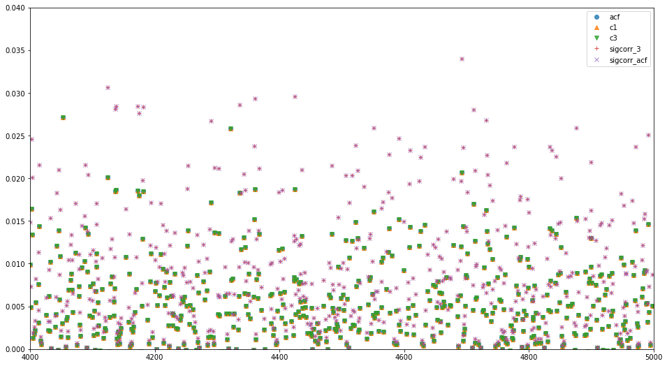
results = pandas.DataFrame({'c1':m1corr, 'c3':m3corr, 'acf':acfcorr, 'sigcorr_acf':sigcorr_acf, 'sigcorr_3':sigcorr_3})
results[4000:].plot(figsize=[16,9],style=['o','^','v','+','x',''],alpha=0.8,ylim=[0,0.04])  # 差が広がるlagが大きい領域のみplot
plt.show()

result

速度の出力(100系列分の合計時間）
scipy.signal.correlation くっそ早いよ

method	result (1回あたりの実行時間は100で除したもの)
corr1	16.3 s ± 137 ms per loop
corr3	12.1 s ± 38.6 ms per loop
acf	6.96 s ± 175 ms per loop
sigcorr_acf	218 ms ± 101 µs per loop
sigcorr_3	220 ms ± 117 µs per loop

$lag>4000$ の領域の相関関数を比較して，特にsigcorrの関数外操作に間違えがないかチェック．
確かに，corr1とacfとsigcorr_arcは等しく，corr3とsigcorr_3も等しい．