KerasでCNN実装

目的

• Kerasの習得
• ニューラルネットワークのさらなる理解
• CNNによるクラス分類と手順を解説

概要

データセット：CIFAR-10
ネットワーク：6層ニューラルネットワーク
実行環境：Google Colaboratory（GPU）

import numpy as np
import pandas as pd
import matplotlib.pyplot as plt
%config InlineBackend.figure_formats = {'png', 'retina'}

import os
from keras.models import Sequential, load_model
from keras.layers.convolutional import Conv2D, MaxPooling2D
from keras.layers.core import Activation, Flatten, Dense, Dropout
from keras.optimizers import Adam, Adagrad, RMSprop, SGD
from keras.utils.np_utils import to_categorical
from keras.callbacks import EarlyStopping, ModelCheckpoint, ReduceLROnPlateau, TensorBoard
from keras.datasets import cifar10

データ取得

(X_train, y_train), (X_test, y_test) = cifar10.load_data()
print(X_train.shape, y_train.shape, X_test.shape, y_test.shape) 

Downloading data from https://www.cs.toronto.edu/~kriz/cifar-10-python.tar.gz
170500096/170498071 [==============================] - 65s 0us/step
(50000, 32, 32, 3) (50000, 1) (10000, 32, 32, 3) (10000, 1)

# データ型の変換＆正規化
X_train = X_train.astype('float32') / 255
X_test = X_test.astype('float32') / 255

# one-hot変換
num_classes = 10 
y_train = to_categorical(y_train, num_classes = num_classes)
y_test = to_categorical(y_test, num_classes = num_classes)

モデル構築

6層ネットワーク
入力層
→Conv + Conv + Pooling + Dropout
→Conv + Conv + Pooling + Dropout
→全結合層 + Dropout
→出力層

model = Sequential()

model.add(Conv2D(
    32, # フィルター数（出力される特徴マップのチャネル）
    kernel_size = 3, # フィルターサイズ
    padding = "same", # 入出力サイズが同じ
    activation = "relu", # 活性化関数
    input_shape = (32, 32, 3) # 入力サイズ
))
model.add(Conv2D(
    32,
    kernel_size = 3,
    activation = "relu"
))
# 各特徴マップのチャネルは変わらず、サイズが1/2
model.add(MaxPooling2D(pool_size = (2, 2)))
model.add(Dropout(0.2))

model.add(Conv2D(
    64,
    kernel_size = 3,
    padding = "same", 
    activation = "relu"
))
model.add(Conv2D(
    64,
    kernel_size = 3,
    activation = "relu"
))
model.add(MaxPooling2D(pool_size = (2, 2)))
model.add(Dropout(0.2))

# 全結合層（fully-connected layers）につなげるため、
# マトリックスデータ（多次元配列）である特徴マップを多次元ベクトルに変換（平坦化）
model.add(Flatten())
# サイズ512のベクトル（512次元ベクトル）を出力
model.add(Dense(512, activation = "relu"))
model.add(Dropout(0.5))
# クラス数のベクトルを出力
model.add(Dense(num_classes))
model.add(Activation("softmax"))

optimizer = Adam(lr = 0.001)
model.compile(
    optimizer = optimizer,
    loss = "categorical_crossentropy",
    metrics = ["accuracy"]
)

モデル要約

model.summary()

________________________________________________________________
Layer (type)                 Output Shape              Param #   
=================================================================
conv2d_1 (Conv2D)            (None, 32, 32, 32)        896       
_________________________________________________________________
conv2d_2 (Conv2D)            (None, 30, 30, 32)        9248      
_________________________________________________________________
max_pooling2d_1 (MaxPooling2 (None, 15, 15, 32)        0         
_________________________________________________________________
dropout_1 (Dropout)          (None, 15, 15, 32)        0         
_________________________________________________________________
conv2d_3 (Conv2D)            (None, 15, 15, 64)        18496     
_________________________________________________________________
conv2d_4 (Conv2D)            (None, 13, 13, 64)        36928     
_________________________________________________________________
max_pooling2d_2 (MaxPooling2 (None, 6, 6, 64)          0         
_________________________________________________________________
dropout_2 (Dropout)          (None, 6, 6, 64)          0         
_________________________________________________________________
flatten_1 (Flatten)          (None, 2304)              0         
_________________________________________________________________
dense_1 (Dense)              (None, 512)               1180160   
_________________________________________________________________
dropout_3 (Dropout)          (None, 512)               0         
_________________________________________________________________
dense_2 (Dense)              (None, 10)                5130      
_________________________________________________________________
activation_1 (Activation)    (None, 10)                0         
=================================================================
Total params: 1,250,858
Trainable params: 1,250,858
Non-trainable params: 0
_________________________________________________________________

Paramの計算
- conv2d_1： 32 × 3 × 3 × 3 ＋ 32 = 896
- conv2d_2： 32 × 3 × 3 × 32 ＋ 32 = 9,248
- conv2d_3： 64 × 3 × 3 × 32 ＋ 64 = 18,496
- conv2d_4： 64 × 3 × 3 × 64 ＋ 64 = 36,928
- dense_1： 2304 × 512 ＋ 512 = 1,180,160
- dense_2： 512 × 10 ＋ 10 = 5,130

モデル学習

# EarlyStopping
early_stopping = EarlyStopping(
    monitor='val_loss',
    patience=10,
    verbose=1
)

# ModelCheckpoint
weights_dir = './weights/'
if os.path.exists(weights_dir) == False:os.mkdir(weights_dir)
model_checkpoint = ModelCheckpoint(
    weights_dir + "val_loss{val_loss:.3f}.hdf5",
    monitor = 'val_loss',
    verbose = 1,
    save_best_only = True,
    save_weights_only = True,
    period = 3
)

# reduce learning rate
reduce_lr = ReduceLROnPlateau(
    monitor = 'val_loss',
    factor = 0.1,
    patience = 3,
    verbose = 1
)

# log for TensorBoard
logging = TensorBoard(log_dir = "log/")

%%time

# モデルの学習
hist = model.fit(
    X_train,
    y_train,
    verbose = 1,
    epochs = 50,
    batch_size = 32,
    validation_split = 0.2,
    callbacks = [early_stopping, reduce_lr, logging]
)

Train on 40000 samples, validate on 10000 samples
Epoch 1/50
40000/40000 [==============================] - 26s 661us/step - loss: 1.5687 - acc: 0.4241 - val_loss: 1.2233 - val_acc: 0.5587
Epoch 2/50
40000/40000 [==============================] - 25s 632us/step - loss: 1.1871 - acc: 0.5787 - val_loss: 1.0178 - val_acc: 0.6412
Epoch 3/50
40000/40000 [==============================] - 25s 614us/step - loss: 1.0248 - acc: 0.6377 - val_loss: 0.8948 - val_acc: 0.6880

〜省略〜

Epoch 00024: ReduceLROnPlateau reducing learning rate to 1.0000000656873453e-06.
Epoch 25/50
40000/40000 [==============================] - 24s 609us/step - loss: 0.3017 - acc: 0.8926 - val_loss: 0.6862 - val_acc: 0.7939
Epoch 26/50
40000/40000 [==============================] - 24s 611us/step - loss: 0.2950 - acc: 0.8949 - val_loss: 0.6863 - val_acc: 0.7939
Epoch 27/50
40000/40000 [==============================] - 25s 621us/step - loss: 0.2993 - acc: 0.8933 - val_loss: 0.6864 - val_acc: 0.7936

Epoch 00027: ReduceLROnPlateau reducing learning rate to 1.0000001111620805e-07.
Epoch 28/50
40000/40000 [==============================] - 25s 619us/step - loss: 0.3022 - acc: 0.8918 - val_loss: 0.6864 - val_acc: 0.7935
Epoch 00028: early stopping
CPU times: user 10min 45s, sys: 1min 56s, total: 12min 41s
Wall time: 11min 29s

モデル保存

model_dir = './model/'
if os.path.exists(model_dir) == False:os.mkdir(model_dir)

model.save(model_dir + 'model.hdf5')

# optimizerのない軽量モデルを保存（学習や評価は不可だが、予測は可能）
model.save(model_dir + 'model-opt.hdf5', include_optimizer = False)

# ベストの重みのみ保存
model.save_weights(weights_dir + 'model_weight.hdf5')

学習曲線をプロット

plt.figure(figsize = (18,6))

# accuracy
plt.subplot(1, 2, 1)
plt.plot(hist.history["acc"], label = "acc", marker = "o")
plt.plot(hist.history["val_acc"], label = "val_acc", marker = "o")
#plt.xticks(np.arange())
#plt.yticks(np.arange())
plt.xlabel("epoch")
plt.ylabel("accuracy")
#plt.title("")
plt.legend(loc = "best")
plt.grid(color = 'gray', alpha = 0.2)

# loss
plt.subplot(1, 2, 2)
plt.plot(hist.history["loss"], label = "loss", marker = "o")
plt.plot(hist.history["val_loss"], label = "val_loss", marker = "o")
#plt.xticks(np.arange())
#plt.yticks(np.arange())
plt.xlabel("epoch")
plt.ylabel("loss")
#plt.title("")
plt.legend(loc = "best")
plt.grid(color = 'gray', alpha = 0.2)

plt.show()

モデル評価

score = model.evaluate(X_test, y_test, verbose=1)
print("evaluate loss: {0[0]}".format(score))
print("evaluate acc: {0[1]}".format(score))

10000/10000 [==============================] - 3s 262us/step
evaluate loss: 0.6986239423751831
evaluate acc: 0.7907

モデル読み込み

model = load_model(model_dir + 'model.hdf5')

# optimaizerがないモデルの場合（予測のみに使用可能）
model = load_model(model_dir + 'model_opt.hdf5', compile = False)

モデル予測

labels = np.array([
   'airplane','automobile','bird','cat','deer','dog','frog','horse','ship','truck'
])

testデータ30件の画像と正解ラベルを出力

# testデータ30件の正解ラベル
true_classes = np.argmax(y_test[0:30], axis = 1)

# testデータ30件の画像と正解ラベルを出力
plt.figure(figsize = (16, 6))
for i in range(30):
    plt.subplot(3, 10, i + 1)
    plt.axis("off")
    plt.title(labels[true_classes[i]])
    plt.imshow(X_test[i])
plt.show()

testデータ30件の画像と予測ラベル＆予測確率を出力

# testデータ30件の予測ラベル
pred_classes = model.predict_classes(X_test[0:30])

# testデータ30件の予測確率
pred_probs = model.predict(X_test[0:30]).max(axis = 1)
pred_probs = ['{:.4f}'.format(i) for i in pred_probs]

# testデータ30件の画像と予測ラベル＆予測確率を出力
plt.figure(figsize = (16, 6))
for i in range(30):
    plt.subplot(3, 10, i + 1)
    plt.axis("off")
    if pred_classes[i] == true_classes[i]:
        plt.title(labels[pred_classes[i]] + '\n' + pred_probs[i])
    else:
        plt.title(labels[pred_classes[i]] + '\n' + pred_probs[i], color = "red")
    plt.imshow(X_test[i])
plt.show()

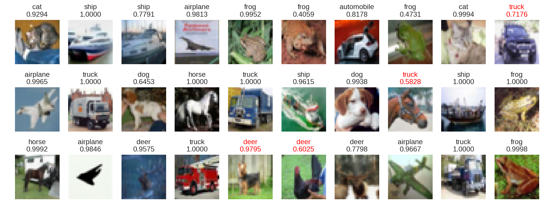
モデル評価でaccuracy 79%、loss 0.69を計測。決して高い精度とは言えない。モデル予測でクラス分類のいくつかに誤りが見られるだけではなく、その誤りが高い確率だったり、正解できていても確率が低かったりしている。ネットワークの改修やハイパーパラメータのチューニングによる検証、さらには既存の学習済みモデルを使ったFine-tuningを試してみたい。

【補足】CIFAR-10以外の外部画像を予測

from PIL import Image
import glob

# 各外部画像のパスを取得
image_paths = glob.glob('img/*.png')
image_paths

['img/cat.png', 'img/dog.png']

画像加工

# 画像を中央でクロップ
def crop_center(pil_img, crop_width, crop_height):
    img_width, img_height = pil_img.size
    return pil_img.crop((
        (img_width - crop_width) // 2,
        (img_height - crop_height) // 2,
        (img_width + crop_width) // 2,
        (img_height + crop_height) // 2
    ))

# 画像リサイズ
def crop_resize(image_path, resize_width, resize_height):
    image = Image.open(image_path)
    crop = crop_center(image, min(image.size), min(image.size))
    resized = crop.resize((resize_width, resize_height))
    img = np.array(resized).astype("float32")
    img /= 255
    return img

images = [crop_resize(p, 32, 32) for p in image_paths]
# 配列に変換
images = np.asarray(images)

外部画像を予測

# 外部画像の正解ラベル
true_classes = np.array([list(labels).index('cat'),list(labels).index('dog')])
print(true_classes)

[3 5]

# 外部画像の予測ラベル
pred_classes = model.predict_classes(images)

# 外部画像の予測確率
pred_probs = model.predict(images).max(axis = 1)
pred_probs = ['{:.4f}'.format(i) for i in pred_probs]

# 外部画像と予測ラベル&予測確率を出力
plt.figure(figsize = (16, 6))
for i in range(2):
    plt.subplot(1, 10, i + 1)
    plt.axis("off")
    if pred_classes[i] == true_classes[i]:
        plt.title(labels[pred_classes[i]] + '\n' + pred_probs[i])
    else:
        plt.title(labels[pred_classes[i]] + '\n' + pred_probs[i], color = "red")
    plt.imshow(images[i])
plt.show()

高い確率でクラス分類できている。