More than 3 years have passed since last update.

Hierarchical clustering in Scipy

Posted at 2020-08-10

Reference

Preparation

import numpy as np
import pandas as pd
import matplotlib.pyplot as plt
import seaborn as sns
%matplotlib inline
plt.rcParams['font.size']=15

def plt_legend_out(frameon=True):
    plt.legend(bbox_to_anchor=(1.05, 1), loc='upper left', borderaxespad=0, frameon=frameon)

from scipy.spatial.distance import pdist
from scipy.spatial.distance import squareform
from scipy.cluster.hierarchy import centroid, fcluster
from scipy.cluster.hierarchy import cut_tree

Data

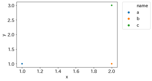
以下のa,b,cを分類することを考えます。

df = pd.DataFrame({'x':[1,2,2],'y':[1,1,3],'name':['a','b','c']})

sns.scatterplot(data=df,x='x',y='y',hue='name')
plt_legend_out()
plt.show()

Main

距離行列を計算します。

>>> y = pdist(df[['x','y']])
>>> y
array([1.        , 2.23606798, 2.        ])

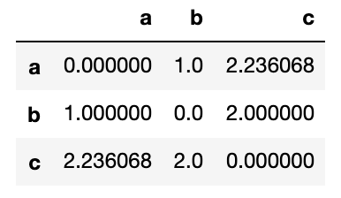
上記の行列は、以下の距離行列の省略形です。

df_plot = pd.DataFrame(squareform(pdist(df[['x','y']])))

df_plot.columns = df['name'].values
df_plot.index   = df['name'].values
df_plot

averageをとってクラスタリングします。

>>> Z = linkage(y, method='average')
>>> Z
array([[0.        , 1.        , 1.        , 2.        ],
       [2.        , 3.        , 2.11803399, 3.        ]])

0.9と1.1がクラスタ数の境目です。

dendrogram(Z,labels=df['name'].values)
plt.axhline(1.1,color='gray',ls='dashed')
plt.axhline(0.9,color='gray',ls='dashed')
plt.ylabel('distance')
plt.show()

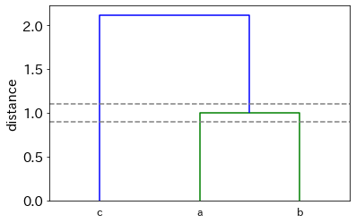
距離に1.1を指定するとクラスタ数は2になり、0.9を指定するとクラスタ数は3になります。

>>> fcluster(Z, 1.1, criterion='distance')
array([1, 1, 2], dtype=int32)

>>> fcluster(Z, 0.9, criterion='distance')
array([1, 2, 3], dtype=int32)

cut_treeでクラスタ数を指定することも可能です。

>>> cut_tree(Z, n_clusters=2)
array([[0],
       [0],
       [1]])

（省略）

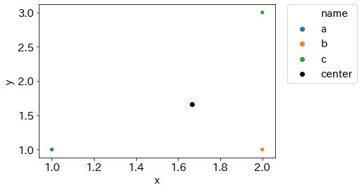
sns.scatterplot(data=df,x='x',y='y',hue='name')
plt.scatter(df['x'].mean(),df['y'].mean(),label='center',color='k')
plt_legend_out()
plt.show()

You get articles that match your needs
You can efficiently read back useful information
You can use dark theme

What you can do with signing up