motivation
データ観察の際、相関係数でデータの傾向を見ることがあります。ただし、外れ値に引っ張られるのが悩みどころです。ロバストで相関係数チックな指標はないのでしょうか。

library
import numpy as np
import pandas as pd
import matplotlib.pyplot as plt
import seaborn as sns
%matplotlib inline
plt.rcParams['font.size']=15

def plt_legend_out(frameon=True):
    plt.legend(bbox_to_anchor=(1.05, 1), loc='upper left', borderaxespad=0, frameon=frameon)
from scipy import stats
from scipy.stats import norm
from scipy.stats import laplace
from scipy.stats import pearsonr
data
np.random.seed(0)
num_data = 20
ratio = 1.5

x1 = np.linspace(1,5,num_data)
noise = np.random.rand(num_data)
x2 = x1 + noise
# x2[20] = x2[20]**2
# x2[int(len(x2)/3)] = x2[len(x2)-1]

max = x2[len(x2)-1]*ratio + 1
min = x2[0] -1

plt.figure(figsize=(8,5))
plt.subplots_adjust(wspace=0.1,hspace=0.1)

plt.subplot(2,2,1)
plt.scatter(x1,x2,color='k')
plt.xlabel('$x_1$')
plt.ylabel('$x_2$')
plt.title('Pearson corr = '+str(np.round(stats.pearsonr(x1,x2)[0],2)))
plt.axvline(norm.fit(x1)[0],label='$\mu_{x_1}$',color='r')
# plt.axvline(norm.fit(x1)[0]+norm.fit(x1)[1],label='$\mu_{x_1}$',color='r',ls='dashed')
plt.axvspan(norm.fit(x1)[0]-norm.fit(x1)[1],norm.fit(x1)[0]+norm.fit(x1)[1],label='$\sigma_{x_1}$',color='r',alpha=0.15)
plt.axhspan(norm.fit(x2)[0]-norm.fit(x2)[1],norm.fit(x2)[0]+norm.fit(x2)[1],label='$\sigma_{x_2}$',color='b',alpha=0.15)
plt.axhline(norm.fit(x2)[0],label='$\mu_{x_2}$',color='b')
plt.ylim([min,max])
plt.xlabel('')
plt.tick_params(bottom=False,labelbottom=False)

plt.subplot(2,2,3)
plt.scatter(x1,x2,color='k')
plt.xlabel('$x_1$')
plt.ylabel('$x_2$')
# plt.title('Spearman corr = '+str(np.round(stats.pearsonr(x1,x2)[0],2)))
plt.axvline(laplace.fit(x1)[0],label='$\mu_{x_1}$',color='r')
# plt.axvline(laplace.fit(x1)[0]+laplace.fit(x1)[1],label='$\mu_{x_1}$',color='r',ls='dashed')
plt.axvspan(laplace.fit(x1)[0]-laplace.fit(x1)[1],laplace.fit(x1)[0]+laplace.fit(x1)[1],label='$\sigma_{x_1}$',color='r',alpha=0.15)
plt.axhspan(laplace.fit(x2)[0]-laplace.fit(x2)[1],laplace.fit(x2)[0]+laplace.fit(x2)[1],label='$\sigma_{x_2}$',color='b',alpha=0.15)
plt.axhline(laplace.fit(x2)[0],label='$\mu_{x_2}$',color='b')
plt.ylim([min,max])

x2[0] = x2[len(x2)-1]*ratio

plt.subplot(2,2,2)
plt.scatter(x1,x2,color='k')
plt.xlabel('$x_1$')
plt.tick_params(left=False,labelleft=False,bottom=False,labelbottom=False)
plt.axvline(norm.fit(x1)[0],label='$\mu_{norm}$',color='r')
# plt.axvline(norm.fit(x1)[0]+norm.fit(x1)[1],label='$\mu_{x_1}$',color='r',ls='dashed')
plt.axvspan(norm.fit(x1)[0]-norm.fit(x1)[1],norm.fit(x1)[0]+norm.fit(x1)[1],label='$\sigma_{norm}$',color='r',alpha=0.15)
plt.axhspan(norm.fit(x2)[0]-norm.fit(x2)[1],norm.fit(x2)[0]+norm.fit(x2)[1],label='$\sigma_{norm}$',color='b',alpha=0.15)
plt.axhline(norm.fit(x2)[0],label='$\mu_{norm}$',color='b')
plt.title('Peason corr = '+str(np.round(stats.pearsonr(x1,x2)[0],2)))
plt.xlabel('')
# plt.suptitle('Spearman corr = '+str(np.round(stats.pearsonr(x1,x2)[0],2)))
plt.ylim([min,max])
plt_legend_out()

plt.subplot(2,2,4)
plt.scatter(x1,x2,color='k')
plt.xlabel('$x_1$')
plt.tick_params(left=False,labelleft=False)
plt.axvline(laplace.fit(x1)[0],label='$\mu_{lap}$',color='r')
# plt.axvline(laplace.fit(x1)[0]+laplace.fit(x1)[1],label='$\mu_{x_1}$',color='r',ls='dashed')
plt.axvspan(laplace.fit(x1)[0]-laplace.fit(x1)[1],laplace.fit(x1)[0]+laplace.fit(x1)[1],label='$\sigma_{lap}$',color='r',alpha=0.15)
plt.axhspan(laplace.fit(x2)[0]-laplace.fit(x2)[1],laplace.fit(x2)[0]+laplace.fit(x2)[1],label='$\sigma_{lap}$',color='b',alpha=0.15)
plt.axhline(laplace.fit(x2)[0],label='$\mu_{lap}$',color='b')
# plt.title('Peason corr = '+str(np.round(stats.pearsonr(x1,x2)[0],2)))
# plt.suptitle('Spearman corr = '+str(np.round(stats.pearsonr(x1,x2)[0],2)))
plt.ylim([min,max])
plt_legend_out()
plt.show()
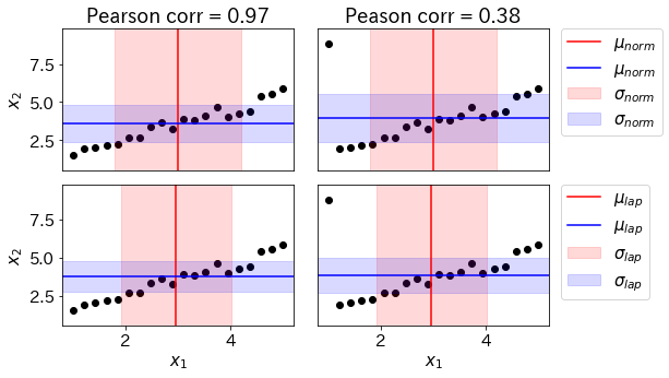
適当な$x_1$と$x_2$を生成します。正規分布とラプラス分布それぞれの$\mu$、$\sigma$を最尤推定で求めます。
correlation coefficient
最尤推定で求めた$\mu$と$\sigma$を、無理やり以下の相関係数の計算式に当てはめてみました。が、こんなことやって良いのかわかりません。
$$
\begin{align*}
r &= \frac{s_{xy}}{s_xs_y} = \frac{\frac{1}{n}\sum_{i=1}^n(x_i-\overline{x})(y_i-\overline{y})}{\sqrt{\frac{1}{n}\sum_{i=1}^n(x_i-\overline{x})^2}\sqrt{\frac{1}{n}\sum_{i=1}^n(y_i-\overline{y})^2}}
\end{align*}
$$
>>> print('normal  :',np.mean((x1 - norm.fit(x1)[0]) * (x2 - norm.fit(x2)[0])) / (np.sqrt(norm.fit(x1)[1])*np.sqrt(norm.fit(x2)[1])))
>>> print('laplace :',np.mean((x1 - laplace.fit(x1)[0]) * (x2 - laplace.fit(x2)[0])) / (np.sqrt(laplace.fit(x1)[1])*np.sqrt(laplace.fit(x2)[1])))
normal  : 0.5224358514430528
laplace : 0.6620999405900793