テンプレートマッチングで物体検出

概要

テンプレートマッチングで物体検出をやってみたいと思います。よくある例は二値画像やマークなので、自然画像で試してみたいと思います。

データ

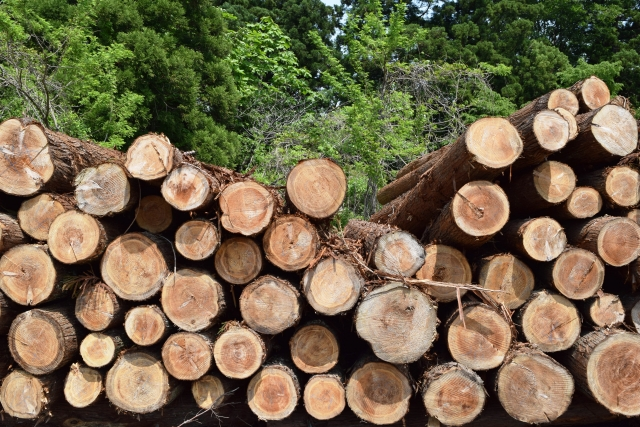
今回は丸太を検出してみようと思います。データはphotoACからダウンロードしました。推論対象画像はこの画像とこの画像のSサイズを使用し、テンプレート画像はこの画像のMサイズからトリミングしました。

推論対象画像1

推論対象画像2

テンプレート画像

プログラム

下記のライブラリをインストールします。

pip install numpy
pip install matplotlib
pip install opencv-python

下記は物体検出を実行するコードです。

main.py

import json

import cv2
import numpy as np
from matplotlib import pyplot as plt


def topk_2d(mat, k):
    idx = np.argpartition(mat.ravel(), mat.size-k)[-k:]
    ys, xs = np.unravel_index(idx, mat.shape)
    return ys, xs


def plot_box(img, boxes):
    result_img = img.copy()
    for box in boxes:
        result_img = cv2.rectangle(
            result_img,
            pt1=box[:2],
            pt2=box[2:],
            color=(255, 0, 0),
            thickness=2)
    return result_img


def nms(boxes, scores, nms_thresh=0.5, top_k=200):
    """
    boxes: np.array([[x1, y1, x2, y2],...])
    """
    keep = []
    if len(boxes) == 0:
        return keep
    x1 = boxes[:, 0]
    y1 = boxes[:, 1]
    x2 = boxes[:, 2]
    y2 = boxes[:, 3]
    area = (x2 - x1) * (y2 - y1)
    idx = np.argsort(scores, axis=0)
    idx = idx[-top_k:]

    while len(idx) > 0:
        last = len(idx)-1
        i = idx[last]  # index of current largest val
        keep.append(i)
        xx1 = np.maximum(x1[i], x1[idx[:last]])
        yy1 = np.maximum(y1[i], y1[idx[:last]])
        xx2 = np.minimum(x2[i], x2[idx[:last]])
        yy2 = np.minimum(y2[i], y2[idx[:last]])

        w = np.maximum(0, xx2 - xx1)
        h = np.maximum(0, yy2 - yy1)

        inter = w * h
        iou = inter / (area[idx[:last]] + area[i] - inter)
        idx = np.delete(idx, np.concatenate(
            ([last], np.where(iou > nms_thresh)[0])))

    return boxes[keep], scores[keep]


def get_candidate_coord(
        res,
        /,
        k=1000,
        threshold=0.5,
        mode='threshold'
):
    if mode == 'threshold':
        ys, xs = np.where(res >= threshold)
    elif mode == 'topk':
        ys, xs = topk_2d(res, k=k)
    else:
        raise ValueError('Wrong mode')
    return ys, xs


def template_match(
        image,
        templ,
        method=cv2.TM_CCOEFF_NORMED,
        threshold=0.5,
        k=1000,
        mode='threshold'
):
    res = cv2.matchTemplate(
        image=image,
        templ=templ,
        method=method
    )
    ys, xs = get_candidate_coord(
        res, k=k, threshold=threshold, mode=mode)

    h, w = templ.shape[:2]
    boxes, scores = [], []
    for x, y in zip(xs, ys):
        box = [x, y, x + w, y + h]
        boxes.append(box)
        scores.append(res[y, x])

    boxes = np.array(boxes)
    scores = np.array(scores)
    return boxes, scores


def detect_boxes(
        template, img, threshold, nms_thresh):
    # 複数のサイズパターンでテンプレートマッチングを行う
    size_candidate = [
        (40, 40),
        (45, 45),
        (50, 50),
        (55, 55),
        (60, 60),
        (65, 65),
        (70, 70),
        (75, 75),
        (80, 80)
    ]
    all_boxes = []
    all_scores = []
    for i_size in size_candidate:
        template_gray_resized = cv2.resize(template, i_size)
        boxes, scores = template_match(
            image=img,
            templ=template_gray_resized,
            method=cv2.TM_CCOEFF_NORMED,
            threshold=threshold
        )
        all_boxes.extend(boxes)
        all_scores.extend(scores)

    all_boxes = np.array(all_boxes)
    all_scores = np.array(all_scores)

    if all_scores.shape[0] <= 0:
        print('No detected')
        return

    all_boxes, all_scores = nms(
        all_boxes, all_scores,
        nms_thresh=nms_thresh, top_k=0)
    return all_boxes, all_scores


def main():
    # テンプレート画像読み込み
    template = cv2.imread('./template.jpg')
    template_gray = cv2.cvtColor(template, cv2.COLOR_BGR2GRAY)

    results, result_imgs = [], []
    filenames = [
        './22456235_s.jpg',
        './25153855_s.jpg'
    ]
    for i, fname in enumerate(filenames):
        # 推論対象画像読み込み
        img = cv2.imread(fname)
        img_gray = cv2.cvtColor(img, cv2.COLOR_BGR2GRAY)

        # 物体検出を実行
        all_boxes, all_scores = detect_boxes(
            template_gray,
            img_gray,
            threshold=0.3,
            nms_thresh=0.1)

        # 検出結果を保存
        for j, (box, score) in enumerate(zip(all_boxes, all_scores)):
            detected_instance = {
                'id': j+1,
                'image_id': i+1,
                'category_id': 1,
                'iscrowd': 0,
                'segmentation': []
            }
            x1, y1, x2, y2 = list(map(int, box))
            detected_instance['bbox'] = [x1, y1, x2 - x1, y2 - y1]
            detected_instance['area'] = (x2 - x1) * (y2 - y1)
            detected_instance['score'] = float(score)
            results.append(detected_instance)

        # Boxを描画する
        result_img = plot_box(img, all_boxes)
        result_img = cv2.cvtColor(result_img, cv2.COLOR_BGR2RGB)
        result_imgs.append(result_img)

    with open('./detections_coco.json', 'w') as f:
        json.dump(results, f, indent=4)

    # Boxを表示する
    for result_img in result_imgs:
        plt.imshow(result_img)
        plt.show()


if __name__ == '__main__':
    main()

OpenCVのmatchTemplateをtemplate_match 関数でラップしています。テンプレートマッチングを実行し、物体を検出した座標をboxesに格納します。cv2.matchTemplateのmethodで指定できる類似度についてはOpenCVのドキュメントを参照してください。

テンプレートマッチングはテンプレート画像と推論対象画像の類似度を計算して物体の位置を検出します。get_candidate_coord関数は類似度が閾値以上、または類似度が上位k個の位置を取得します。topk_2dは2次元配列から上位k個のインデックスを取得する関数です。

nms関数はNMS (Non-Maximum Suppression)を実行する関数です。テンプレートマッチングはテンプレートを推論対象画像上にスライドさせて物体位置を特定するため、物体がある場所に複数のボックスを検出しやすいです。したがって、重複するボックスを排除することが必要となります。

detect_boxes関数はファサードです。テンプレート画像のサイズを複数パターン変えてテンプレートマッチングを行っています。他にも明度や回転などのパターンを変えてテンプレートマッチングをすることが考えられます。ただし、パターンが増えるほど処理回数が増えるので時間がかかるようになります。

plot_box関数は、画像に検出したボックスを描く関数です。

また、main関数では物体検出を実行後、ボックスの検出結果をCOCOフォーマットでファイルに出力しています。

検出結果

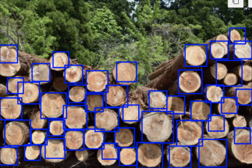
検出結果(画像1)

検出結果(画像2)

今回は類似度の閾値を0.3、NMSの閾値を0.1としました。これらの閾値に敏感に結果が変わるので、本来は閾値を何らかの方法で最適化する必要があります。今回は簡易的に手動で決めました。

実行時間は1~2秒程度でした。類似度の閾値を小さくすると検出数が増えるので、NMSの実行時間が$ \mathcal{O}(N^2)$で増えることに注意してください。

精度を評価します。物体検出の評価指標を計算するライブラリを導入します。

pip install object_detection_metrics
pip install shapely 

True PositiveのIoU閾値は0.5とします。今回は類似度の閾値を決めているので、Precision および Recallで評価します。

精度は次のコードで計算できます。

eval.py

from podm import coco_decoder
from podm.metrics import get_bounding_boxes, get_pascal_voc_metrics

with open('annotations/instances_default.json') as fp:
    gold_dataset = coco_decoder.load_true_object_detection_dataset(fp)

with open('detections_coco.json') as fp:
    pred_dataset = coco_decoder.load_pred_object_detection_dataset(
        fp, gold_dataset)

gt_BoundingBoxes = get_bounding_boxes(gold_dataset)
pd_BoundingBoxes = get_bounding_boxes(pred_dataset)
results = get_pascal_voc_metrics(gt_BoundingBoxes, pd_BoundingBoxes, .5)

for category, metric in results.items():
    label = metric.label
    print('tp', metric.tp)
    print('fp', metric.fp)
    print('fn', metric.num_groundtruth - metric.tp)
    print('precision', metric.precision[-1])
    print('recall', metric.recall[-1])

精度は下記のようになりました。

	real_pos	real_neg
pred_pos	tp = 90	fp = 12
pred_neg	fn = 43	-

Precision@IoU=0.5,conf=0.3,nms=0.1	Recall@IoU=0.5,conf=0.3,nms=0.1
88.2	67.7

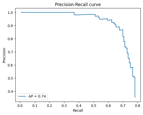
APを計算する場合

APを計算する場合は類似度の閾値を$-1$にします。さらに通常はそれぞれの画像に対するボックスをスコア順で上位$K$にフィルターしますが、今回は$K=\infty$としました。

Precision-Recall 曲線を表示するためにscikit-learnを使用します。

pip install -U scikit-learn

下記は評価のコードです。

eval.py

from matplotlib import pyplot as plt
from podm import coco_decoder
from podm.metrics import get_bounding_boxes, get_pascal_voc_metrics, MetricPerClass
from sklearn.metrics import PrecisionRecallDisplay

with open('annotations/instances_default.json') as fp:
    gold_dataset = coco_decoder.load_true_object_detection_dataset(fp)

with open('detections_coco.json') as fp:
    pred_dataset = coco_decoder.load_pred_object_detection_dataset(
        fp, gold_dataset)

gt_BoundingBoxes = get_bounding_boxes(gold_dataset)
pd_BoundingBoxes = get_bounding_boxes(pred_dataset)
results = get_pascal_voc_metrics(gt_BoundingBoxes, pd_BoundingBoxes, .5)

for category, metric in results.items():
    label = metric.label
    print('ap', metric.ap)

    display = PrecisionRecallDisplay(
        recall=metric.recall,
        precision=metric.precision,
        average_precision=metric.ap,
    )
    display.plot()
    _ = display.ax_.set_title("Precision-Recall curve")
    plt.show()

AP@IoU=0.5, nms=0.1, [tex: K=infty]
73.8

Precision-Recall 曲線

Reference