QuantX SDKで結果を可視化してみる
QuantX SDKを使ってバックテスト結果を見やすくしてみます。
自己紹介
理系大学で、統計を専攻しています。
pythonは初心者で、金融に関してはファイナンスを少しかじってました。smart tradeでインターン中。
目的
アルゴリズムを作ってみたのは良いものの、パラメータの調整とか何回もバックテストしなきゃ...めんどくさい...
たくさんやったバックテストの結果をまとめて表示してくれないかな...
あわよくばその結果の解釈もやってほしいですが、今回は表示までやりたいと思います。
準備
Google colaboratory上でQuantX SDKを使います。
QuantX SDKを使うならこちらの記事が参考になります。
Google Colaboratory上で行うQuantX-SDK事始め
https://qiita.com/katakyo/items/ac01dcd6c692c3585596
プロジェクトの作成やハッシュ番号の取得まではできている前提で進めたいと思います。
また描画に必要なライブラリのmatplotlib、seabornも使います。
実際に実装してみる
2つ実装例を書きました。
扱うアルゴリズムはこちらです。
前回自分で作ったアルゴリズムを色々いじってみたいと思います。
例1:パラメータの調整
今回用いたアルゴリズムのパラメータのうち、ボリンジャーバンドの幅であるsigmaと、ボリンジャーバンドの幅を何日分の分散を使って計算するのかを表すtimeperiodを変えて、どの値を使うのが良いのか模索していきます。
テンプレート
TA-Lib内で、sigmaとtimeperiodを指定する箇所があるので、そこ以外をテンプレート化しました。(見づらいかもしれませんが、コメントアウトした部分の直下にあります。)
my_template = """

import pandas as pd
import talib as ta
import numpy as np

def judge_expand(ar_upperband,ar_lowerband,m):

	ar_volatility = ar_upperband - ar_lowerband
	list_vol = ar_volatility.tolist()
	list_status = [0]*len(list_vol)

	for i in range(m,len(list_vol)):
	  if list_vol[i] > 3*min(list_vol[i-m:i]):
	    list_status[i]=1
	return np.array(list_status)


def judge_plus_two_sigma(sr_upperband,sr_price):
  ar_a = np.greater(sr_price,sr_upperband)
  return ar_a.astype(int)


def judge_minus_two_sigma(sr_lowerband,sr_price):
	ar_a = np.less(sr_price,sr_lowerband)
	return ar_a.astype(int)


def initialize(ctx):
    ctx.logger.debug("initialize() called")
    ctx.codes = [
      2170,2181,2412,3636,4716,6098,6194,6550,1963,6366,6330,1357
      ]
    ctx.symbol_list  = ["jp.stock.{}".format(code) for code in ctx.codes]
    ctx.configure(
      target="jp.stock.daily",
      channels={          # 利用チャンネル
        "jp.stock": {
          "symbols": ctx.symbol_list,
          "columns": [
            "close_price",        # 終値
            "close_price_adj",    # 終値(株式分割調整後)
            "volume_adj",         # 出来高
            "txn_volume",         # 売買代金
          ]
        }
      }
    )


    def _original_signal(pn_data):

      df_cp = pn_data["close_price_adj"].fillna(method="ffill")
      dict_upperband = {}
      dict_middleband = {}
      dict_lowerband = {}
      df_buy_sig = pd.DataFrame(data=0,columns=[], index=df_cp.index)
      df_sell_sig = pd.DataFrame(data=0,columns=[], index=df_cp.index)
      df_ex_buy_sig = pd.DataFrame(data=0,columns=[], index=df_cp.index)
      df_ex_sell_sig = pd.DataFrame(data=0,columns=[], index=df_cp.index)
      df_uband = pd.DataFrame(data=0,columns=[], index=df_cp.index)
      df_lband = pd.DataFrame(data=0,columns=[], index=df_cp.index)
      df_expand = pd.DataFrame(data=0,columns=[], index=df_cp.index)
      df_minus_two_sigma = pd.DataFrame(data=0,columns=[], index=df_cp.index)
      df_plus_two_sigma = pd.DataFrame(data=0,columns=[], index=df_cp.index)

# この後に{{}}で囲まれている部分がパラメータです。
      for sym in df_cp.columns.values:
        dict_upperband[sym], dict_middleband[sym], dict_lowerband[sym] = ta.BBANDS(df_cp[sym].values.astype(np.double),
          timeperiod={{timeperiod}},
          nbdevup={{up_sigma}},
          nbdevdn={{dn_sigma}},
          matype=0)

        df_lband[sym] = dict_lowerband[sym]
        df_uband[sym] = dict_upperband[sym]

        df_expand[sym] = judge_expand(dict_upperband[sym],dict_lowerband[sym],50)
        df_minus_two_sigma[sym] = judge_minus_two_sigma(df_lband[sym],df_cp[sym])
        df_plus_two_sigma[sym] = judge_plus_two_sigma(df_uband[sym],df_cp[sym])

        df_buy_sig[sym] = df_minus_two_sigma[sym] - df_minus_two_sigma[sym]*df_expand[sym]
        df_sell_sig[sym] = df_plus_two_sigma[sym] - df_plus_two_sigma[sym]*df_expand[sym]
        df_ex_buy_sig[sym] = df_plus_two_sigma[sym]*df_expand[sym]
        df_ex_sell_sig[sym] = df_minus_two_sigma[sym]*df_expand[sym]

      return {
        "upperband:price": df_uband,
        "lowerband:price": df_lband,
        "buy:sig": df_buy_sig,
        "sell:sig": df_sell_sig,
        "exbuy:sig":df_ex_buy_sig,
        "exsell:sig":df_ex_sell_sig,

      }
    ctx.regist_signal("original", _original_signal)

def handle_signals(ctx, date, df_current):

  for sym in df_current.index:
    if df_current.loc[sym,"buy:sig"] == 1:
      sec = ctx.getSecurity(sym)
      sec.order_target_percent(0.15, comment="シグナル買" )
    elif df_current.loc[sym,"exbuy:sig"] == 1:
      sec = ctx.getSecurity(sym)
      sec.order_target_percent(0.15, comment="エキスパンドシグナル買")
    elif df_current.loc[sym,"sell:sig"] == 1:
      sec = ctx.getSecurity(sym)
      sec.order_target_percent(0, comment="シグナル売" )
    elif df_current.loc[sym,"exsell:sig"] == 1:
      sec = ctx.getSecurity(sym)
      sec.order_target_percent(0, comment="エキスパンドシグナル売")

    pass
"""
実際にバックテストを行うコード
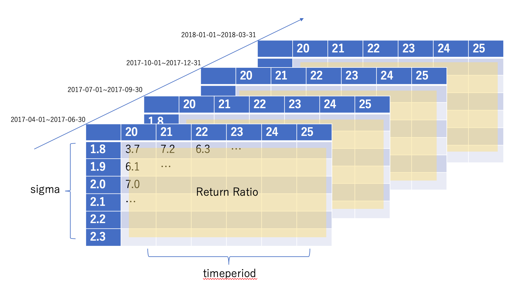
変えるパラメータであるtimeperiod、sigmaを、変える範囲でリスト化します。sigmaは1.8~2.3で0.1ごとに刻んでいます。timeperiodは20日~25日です。また、バックテストは2017年度3ヶ月ごとの4期間を行いました。値はこのアルゴリズムのポートフォリオ全体の損益比としています。
最終的に以下のようなpandasのPanelデータを返します。
from jinja2 import Template
test_hash = ''#取得しているハッシュ番号

# 変化させるパラメータ・回すバックテスト期間の用意
timeperiod_list = [20,21,22,23,24,25]#変化させるtimeperiodのリスト
sigma_list = [1.8,1.9,2.0,2.1,2.2,2.3]#変化させるsigmaのリスト
list_backtest_span_s = ['2017-04-01','2017-07-01','2017-10-01','2018-01-01']#バックテスト開始日のリスト
list_backtest_span_b = ['2017-06-30','2017-09-30','2017-12-31','2018-03-31']#バックテスト終了日のリスト
result_dict={}

# バックテスト期間を変えて繰り返す
for i in range(len(list_backtest_span_s)):
  return_df = pd.DataFrame(data = 0 ,index = sigma_list, columns=[])#sigma*timeperiodのデータフレームの準備

  #timeperiodを変えて繰り返す
  for timeperiod_i in timeperiod_list:
    return_ratio = []#ポートフォリオのリターンを入れるリストを用意する

    #sigmaを変えて繰り返す
    for sigma_i in sigma_list:
      par = {'timeperiod':timeperiod_i,'up_sigma':sigma_i,'dn_sigma':sigma_i}#変えるパラメータを辞書形式で用意
      source = Template(my_template).render(par)#テンプレートに埋め込む

      #バックテストの期間・エンジン・初期保有額を指定する
      bt_parameter = {
          'engine': 'maron-0.0.1b',
          'from_date': list_backtest_span_s[i],
          'to_date': list_backtest_span_b[i],
          'capital_base': 10000000}

      #バックテストの実行・サマリーの取得
      test = qx.project(test_hash)
      test.upload_source(source)
      bt = test.backtest(bt_parameter)
      join = bt.join()
      summary = join.summary()

      #先に用意したreturn_ratioのリストに、バックテストで得られたポートフォリオのリターンを格納する。
      return_ratio.append(float(summary['ReturnRatio']))

    #return_ratioのリストをデータフレームに入れていく。
    return_df[timeperiod_i] = return_ratio

  #バックテスト期間ごとに、データフレームをまとめて辞書にする。
  result_dict[list_backtest_span_s[i]]=return_df

# 最後に用意した辞書をデータフレームに変換
result_panel = pd.Panel(result_dict)
最後に描画するコードです
上記で作成したpanelをグラフに描画します。
今回は結果をわかりやすくするためにヒートマップを作成します。縦軸にボリンジャーバンドの幅であるsigma、横軸にボリンジャーバンドを計算する際に何日分の分散の平均を使うかを表すtimeperiodをとります。
from matplotlib import pyplot as plt
import seaborn as sns

plt.figure(figsize = (20,5))
for i in range(len(list_backtest_span_s)):
  plt.subplot(1,4,i+1)
  sns.heatmap(result_panel[list_backtest_span_s[i]],annot = True, center = 0)
  plt.xlabel('timeperiod')
  plt.ylabel('sigma')
  plt.title(list_backtest_span_s[i]+'~'+list_backtest_span_b[i])
結果
出力結果はこちらです。
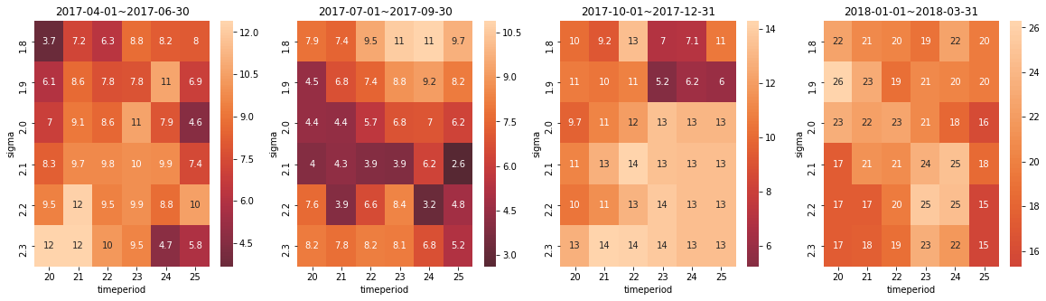
明るいところを見ると、各時期でバラバラですね...
コンスタントに高い利益をあげるパラメータの組み合わせは存在しないということでしょうか...
例2:銘柄ごとの比較
次は、エクスパンドを判定する期間の銘柄ごとに比較していきたいと思います。
エクスパンドを判定する期間が短いほど、急激なエクスパンドを判定しやすくなります。銘柄によってエクスパンションの仕方に特徴があると踏んで、銘柄ごとにこの判定の日数を模索していきます。
テンプレート2
エクスパンドを判定する日数expand_judgeをパラメータとし、そこ以外をテンプレート化しました。(見づらいかもしれませんが、コメントアウトした部分の直下にあります。)
my_template = """

import pandas as pd
import talib as ta
import numpy as np

def judge_expand(ar_upperband,ar_lowerband,m):

	ar_volatility = ar_upperband - ar_lowerband
	list_vol = ar_volatility.tolist()
	list_status = [0]*len(list_vol)

	for i in range(m,len(list_vol)):
	  if list_vol[i] > 3*min(list_vol[i-m:i]):
	    list_status[i]=1
	return np.array(list_status)


def judge_plus_two_sigma(sr_upperband,sr_price):
  ar_a = np.greater(sr_price,sr_upperband)
  return ar_a.astype(int)


def judge_minus_two_sigma(sr_lowerband,sr_price):
	ar_a = np.less(sr_price,sr_lowerband)
	return ar_a.astype(int)


def initialize(ctx):
    ctx.logger.debug("initialize() called")
    ctx.codes = [
      2170,2181,2412,3636,4716,6098,6194,6550,1963,6366,6330,1357
      ]
    ctx.symbol_list  = ["jp.stock.{}".format(code) for code in ctx.codes]
    ctx.configure(
      target="jp.stock.daily",
      channels={          # 利用チャンネル
        "jp.stock": {
          "symbols": ctx.symbol_list,
          "columns": [
            "close_price",        # 終値
            "close_price_adj",    # 終値(株式分割調整後)
            "volume_adj",         # 出来高
            "txn_volume",         # 売買代金
          ]
        }
      }
    )


    def _original_signal(pn_data):

      df_cp = pn_data["close_price_adj"].fillna(method="ffill")
      dict_upperband = {}
      dict_middleband = {}
      dict_lowerband = {}
      df_buy_sig = pd.DataFrame(data=0,columns=[], index=df_cp.index)
      df_sell_sig = pd.DataFrame(data=0,columns=[], index=df_cp.index)
      df_ex_buy_sig = pd.DataFrame(data=0,columns=[], index=df_cp.index)
      df_ex_sell_sig = pd.DataFrame(data=0,columns=[], index=df_cp.index)
      df_uband = pd.DataFrame(data=0,columns=[], index=df_cp.index)
      df_lband = pd.DataFrame(data=0,columns=[], index=df_cp.index)
      df_expand = pd.DataFrame(data=0,columns=[], index=df_cp.index)
      df_minus_two_sigma = pd.DataFrame(data=0,columns=[], index=df_cp.index)
      df_plus_two_sigma = pd.DataFrame(data=0,columns=[], index=df_cp.index)

      for sym in df_cp.columns.values:
        dict_upperband[sym], dict_middleband[sym], dict_lowerband[sym] = ta.BBANDS(df_cp[sym].values.astype(np.double),
          timeperiod=23,
          nbdevup=1.7,
          nbdevdn=1.7,
          matype=0)

        df_lband[sym] = dict_lowerband[sym]
        df_uband[sym] = dict_upperband[sym]

# この後に{{}}で囲まれている部分がパラメータです。
        df_expand[sym] = judge_expand(dict_upperband[sym],dict_lowerband[sym],{{expand_judge}})
        df_minus_two_sigma[sym] = judge_minus_two_sigma(df_lband[sym],df_cp[sym])
        df_plus_two_sigma[sym] = judge_plus_two_sigma(df_uband[sym],df_cp[sym])

        df_buy_sig[sym] = df_minus_two_sigma[sym] - df_minus_two_sigma[sym]*df_expand[sym]
        df_sell_sig[sym] = df_plus_two_sigma[sym] - df_plus_two_sigma[sym]*df_expand[sym]
        df_ex_buy_sig[sym] = df_plus_two_sigma[sym]*df_expand[sym]
        df_ex_sell_sig[sym] = df_minus_two_sigma[sym]*df_expand[sym]

      return {
        "upperband:price": df_uband,
        "lowerband:price": df_lband,
        "buy:sig": df_buy_sig,
        "sell:sig": df_sell_sig,
        "exbuy:sig":df_ex_buy_sig,
        "exsell:sig":df_ex_sell_sig,

      }
    ctx.regist_signal("original", _original_signal)

def handle_signals(ctx, date, df_current):

  for sym in df_current.index:
    if df_current.loc[sym,"buy:sig"] == 1:
      sec = ctx.getSecurity(sym)
      sec.order_target_percent(0.15, comment="シグナル買" )
    elif df_current.loc[sym,"exbuy:sig"] == 1:
      sec = ctx.getSecurity(sym)
      sec.order_target_percent(0.15, comment="エキスパンドシグナル買")
    elif df_current.loc[sym,"sell:sig"] == 1:
      sec = ctx.getSecurity(sym)
      sec.order_target_percent(0, comment="シグナル売" )
    elif df_current.loc[sym,"exsell:sig"] == 1:
      sec = ctx.getSecurity(sym)
      sec.order_target_percent(0, comment="エキスパンドシグナル売")

    pass
"""
実際にバックテストを行うコード
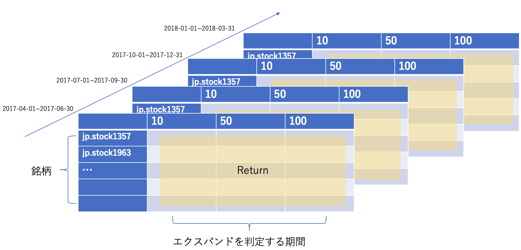
変えるパラメータであるexpand_judgeを、変える範囲でリスト化します。今回は10日、50日、100日の3パターンを用意しました。また、バックテストは2017年度3ヶ月ごとの4期間を行いました。値は各銘柄のリターンとしています。
最終的に以下のようなpandasのPanelデータを返します。
例1のコードと構造はほとんど変わらないです。最後に出力する内容だけが異なるだけです。
from jinja2 import Template
test_hash = ''#取得しているハッシュ番号

expand_judge_list = [10,50,100]

list_backtest_span_s = ['2017-04-01','2017-07-01','2017-10-01','2018-01-01']
list_backtest_span_b = ['2017-06-30','2017-09-30','2017-12-31','2018-03-31']
result_dict={}
for i in range(len(list_backtest_span_s)):
  return_df = pd.DataFrame(data = 0 ,index = [], columns =[] )
  for expand_judge_i in expand_judge_list:
    par = {'expand_judge':expand_judge_i}
    source2 = Template(my_template).render(par)
    bt_parameter = {
        'engine': 'maron-0.0.1b',
        'from_date': list_backtest_span_s[i],
        'to_date': list_backtest_span_b[i],
        'capital_base': 10000000}
    test = qx.project(test_hash)
    test.upload_source(source2)
    bt = test.backtest(bt_parameter)
    join = bt.join()
    summary = join.symbol_summary()
    return_df[expand_judge_i] = summary['return']
  return_df.index = summary['symbol']
  result_dict[list_backtest_span_s[i]]=return_df
result_panel = pd.Panel(result_dict)
最後に描画するコードです
上記で作成したpanelをグラフに描画します。
例1と同様にヒートマップを作成します。
今回は縦軸に銘柄、横軸にexpand_judgeをとります。
from matplotlib import pyplot as plt
import seaborn as sns

list = []
plt.figure(figsize = (15,10))
plt.subplots_adjust(wspace=0.5,hspace=0.35)

for i in range(len(list_backtest_span_s)):
  plt.subplot(2,2,i+1)
  sns.heatmap(result_panel[list_backtest_span_s[i]],annot = True)
  plt.xlabel('expand judge')
  plt.ylabel('Brand number')
  plt.title(list_backtest_span_s[i]+'~'+list_backtest_span_b[i])
結果
特定の銘柄が、コンスタントに利益をあげるようなパラメータの値はありますかね...
強いて言えばjp.stock6194に対して100日でのエクスパンド判定を行うと、ある程度コンスタントに利益が出るのか...
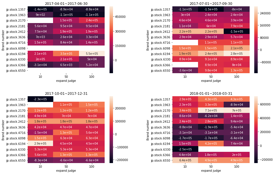
この分析は、業界ごとに銘柄をまとめて行うとヒートマップの特徴を活かせるのではないでしょうか?
業界ごとにエクスパンドに特徴がありそうなので...
最後に
色々できそうですね。
今は目で見て比較するだけですが、その解釈の実装もある程度行なっていきたいと思います。
コードの汚さも、今後洗練させていきます()
誰でも分析できるようなテンプレートみたいなものも今後用意する予定です。
それでは今回はここまで
勉強会の宣伝
SmartTrade社では毎週水曜日18:00から勉強会を行っています。(https://python-algo.connpass.com/)
免責注意事項
このコードや知識を使った実際の取引で生じた損益に関しては一切の責任を負いかねますので御了承下さい