はじめに
ニューラルネットワークの学習では、誤差逆伝播法と呼ばれる手法で各ニューロンの重みの更新を行います。実際に重みの更新を可視化している記事が少なかったので、アニメーションとして可視化を行いました。
環境
- Google Colaboratory Pro
コード
モジュールのimport・変換前のデータ
import torchvision.transforms as transforms
from torch.utils.data import DataLoader
from torchvision.datasets import MNIST
import torch
from torch.autograd import Variable
import torch.nn as nn
import torch.nn.functional as F
import torch.optim as optim
from torch.cuda import device_of
import numpy as np
import pandas as pd
import matplotlib.pyplot as plt
from matplotlib.collections import LineCollection
from matplotlib.animation import FuncAnimation
from matplotlib import rc
import matplotlib
from matplotlib import patches
from scipy.cluster.hierarchy import linkage, dendrogram, fcluster
データとしてMNISTを使用します。
mnist_data = MNIST("./data", train=True, download = True, transform = transforms.ToTensor())
data_loader = DataLoader(mnist_data,
                         batch_size=4,
                         shuffle=False)
データを確認します。
data_iter = iter(data_loader)
images, labels = data_iter.next()

plt.imshow(images[0].numpy().reshape((28,28)), cmap="gray")

データを学習(train)、検証(validation)、テストデータ(test)に分割します。
BATCH_SIZE = 16

trainval_data = MNIST("./data",
                   train=True,
                   download=True,
                   transform=transforms.ToTensor())

test_data = MNIST("./data",
                   train=False,
                   download=True,
                   transform=transforms.ToTensor())

n_trainval_data = len(trainval_data)
train_size = int(n_trainval_data * 0.8)
val_size = n_trainval_data - train_size
train_data, val_data = torch.utils.data.random_split(trainval_data, [train_size, val_size])

train_loader = DataLoader(train_data,
                          batch_size=BATCH_SIZE,
                          shuffle=True)

val_loader = DataLoader(val_data,
                          batch_size=BATCH_SIZE,
                          shuffle=True)

test_loader = DataLoader(test_data,
                          batch_size=BATCH_SIZE,
                          shuffle=True)

print("train data size: ",len(train_data))
print("train iteration number: ",len(train_data)//BATCH_SIZE)
print("val data size: ",len(val_data))
print("val iteration number: ",len(val_data)//BATCH_SIZE)
print("test data size: ",len(test_data))
実行結果
train data size:  48000
train iteration number:  3000
val data size:  12000
val iteration number:  750
test data size:  10000
ニューラルネットワークを生成します。後程第2層から第5層までを可視化します。
class Net(nn.Module):
  def __init__(self):
    super().__init__()
    self.l1 = nn.Linear(28 * 28, 1000)
    self.l2 = nn.Linear(1000, 100)
    self.l3 = nn.Linear(100, 10)
    self.l4 = nn.Linear(10, 10)
    self.l5 = nn.Linear(10, 10)
    self.relu = nn.ReLU()
    self.dropout = nn.Dropout(0.2)

  def forward(self, x):
    x = x.view(-1, 28 * 28)
    x = self.l1(x)
    x = self.relu(x)
    x = self.dropout(x)
    x = self.l2(x)
    x = self.relu(x)
    x = self.l3(x)
    x = self.relu(x)
    x = self.l4(x)
    x = self.relu(x)
    x = self.l5(x)
    return x
device = torch.device("cuda:0" if torch.cuda.is_available() else "cpu")
print(device)

net = Net().to(device)
print(net)
def cal_acc(labels, outputs):
  pred = torch.argmax(outputs, dim=1)
  return torch.sum(labels == pred)
データ量が多いので1エポックのみ学習を行います。バッチサイズは16です。
criterion = nn.CrossEntropyLoss()
optimizer = optim.Adam(net.parameters(), lr=0.001)

history = {"train_loss": [],
            "train_acc": [],
            "val_loss": [],
            "val_acc": [],
            "l1": [],
            "l2": [],
            "l3": [],
            "l4": [],
            "l5": []
            }

for epoch in range(1):
  train_loss = 0
  train_acc = 0
  val_loss = 0
  val_acc = 0

  net.train()
  for i, data in enumerate(train_loader):
    history["l1"].append(net.state_dict()["l1.weight"].to("cpu"))
    history["l2"].append(net.state_dict()["l2.weight"].to("cpu"))
    history["l3"].append(net.state_dict()["l3.weight"].to("cpu"))
    history["l4"].append(net.state_dict()["l4.weight"].to("cpu"))
    history["l5"].append(net.state_dict()["l5.weight"].to("cpu"))
    inputs, labels = data[0].to(device), data[1].to(device)
    optimizer.zero_grad()
    outputs = net(inputs)
    loss = criterion(outputs, labels)
    loss.backward()
    optimizer.step()
    train_loss += loss.item()
    train_acc += cal_acc(labels, outputs)
    if i % ((len(train_data)//BATCH_SIZE)/1000) == ((len(train_data)//BATCH_SIZE)/1000) - 1:
      print(f"epoch:{epoch+1}  index:{(i+1)*BATCH_SIZE}  train_loss:{train_loss/len(inputs):.5f}   train_acc:{train_acc/len(inputs):.5f}")
    history["train_loss"].append(train_loss/len(inputs))
    history["train_acc"].append(train_acc/len(inputs))
    train_loss = 0
    train_acc = 0

  net.eval()
  with torch.no_grad():
    for i, data in enumerate(val_loader):
      inputs, labels = data[0].to(device), data[1].to(device)
      outputs = net(inputs)
      loss = criterion(outputs, labels)
      val_loss += loss.item()
      val_acc += cal_acc(labels, outputs)
      if i % (len(val_data)//BATCH_SIZE) == len(val_data)//BATCH_SIZE - 1:
        print(f"epoch:{epoch+1}  index:{i+1}  val_loss:{val_loss/len(val_data):.5f}  val_acc:{val_acc/len(val_data):.5f}")
        history["val_loss"].append(val_loss/len(val_data))
        history["val_acc"].append(val_acc/len(val_data))
        val_loss = 0
        val_acc = 0
実行結果
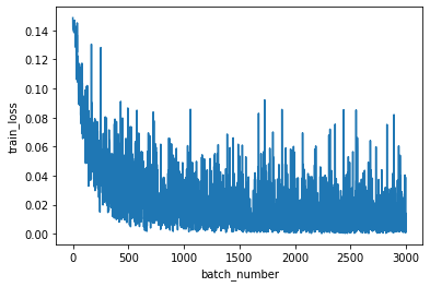
epoch:1 index:320 train_loss:0.14255 train_acc:0.00000
epoch:1 index:640 train_loss:0.14517 train_acc:0.00000
epoch:1 index:960 train_loss:0.11681 train_acc:0.37500
~~~(省略)~~~
epoch:1 index:47680 train_loss:0.00366 train_acc:1.00000
epoch:1 index:48000 train_loss:0.03853 train_acc:0.87500
epoch:1 index:750 val_loss:0.00945 val_acc:0.95625
損失の推移を確認します。
plt.figure()
plt.plot(history["train_loss"])
Qiitaに投稿可能なアニメーション(gifファイル)の容量制限で、100バッチまでの結果を可視化します。
layer_lists = ["l2", "l3", "l4", "l5"]
weight_lists = []
for layer in layer_lists[1:]:
  layer_weight = []
  for i in history[layer]:
    layer_weight.append(i.detach().numpy())
  weight_lists.append(layer_weight)

weight_histories = []
for list_weight in weight_lists:
  trans_history = []
  for i, weights in enumerate(list_weight[0]):
    trans_history.append([])
    for j in range(len(weights)):
      trans_history[i].append([])
  for batch_list in list_weight:
    for i, weights in enumerate(batch_list):
      for j, weight in enumerate(weights):
        trans_history[i][j].append(np.array(weight))
  weight_histories.append(np.array(trans_history))

weight_changes = []
for history_weight in weight_histories:
  change_weight = []
  for i, weight_list in enumerate(history_weight):
    change_weight.append([])
    for j in range(len(weight_list)):
      change_weight[i].append([])
      for k in range(len(history_weight[i][j])):
        if k > 1:
          change_weight[i][j].append(history_weight[i][j][k] - history_weight[i][j][k-1])
  weight_changes.append(np.array(change_weight))
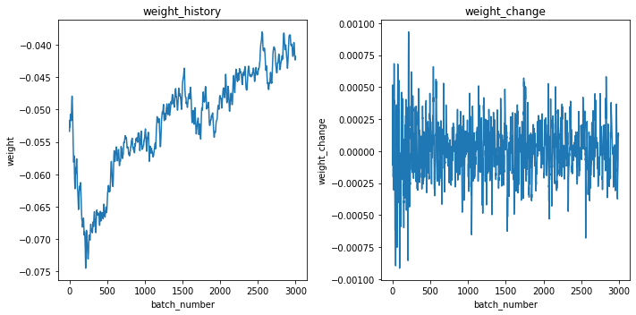
重みの推移と重みの変動(1バッチ前からどのくらい変動したか)を可視化します。
fig = plt.figure(figsize = (10,5))

ax1 = fig.add_subplot(1, 2, 1)
ax1.plot(weight_histories[0][0][0])
ax1.set_xlabel("batch_number")
ax1.set_ylabel("weight")
ax1.set_title("weight_history")

ax2 = fig.add_subplot(1, 2, 2)
ax2.plot(weight_changes[0][0][0])
ax2.set_xlabel("batch_number")
ax2.set_ylabel("weight_change")
ax2.set_title("weight_change")

fig.tight_layout()
plt.show()
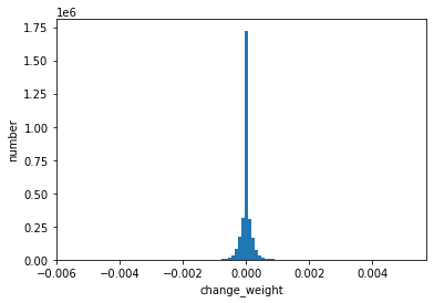
重みの変動がどのように分布するか確認します。
flat_weight_changes = [i.flatten() for i in weight_changes]
plt.hist(flat_weight_changes[0], bins=100)
以降、アニメーション作成のコードを記述しています。行っていることは以下の2点です。
- 視覚化する重み変動の閾値設定(各層における全ての重み変動の中で、上位0.01%の重み変動を可視化する。上位0.01%以外は色の濃さで表現する)
- アニメーションの各フレームの描写
nodes = [history[layer][0].size()[0] for i,layer in enumerate(layer_lists)]

max_node = max(nodes)
positions = []
for index, node in enumerate(nodes):
  pos = []
  for i in range(node):
    pos.append([index,(i/(node-1))*max_node])
  positions.append(pos)

tuples = [tuple(pos) for position in positions for pos in position]

weight_change_abssorts = [np.sort(np.abs(i - np.average(i)))[::-1] for i in flat_weight_changes]
min_weightnum = min([len(weight_change_abssort) for weight_change_abssort in weight_change_abssorts])
tf_lists = [i[int(min_weightnum * 0.0001 *(len(i)/min_weightnum)**(1/2))] for i in weight_change_abssorts]
ave_lists = [np.average(i) for i in flat_weight_changes]
def create_colors(weight_changes, batch, tf_lists, ave_lists):
  colors = []
  for flat_weight_change, tf, ave in zip(weight_changes, tf_lists, ave_lists):
    for i, weight_n1 in enumerate(flat_weight_change):
      for j, weight_hist in enumerate(weight_n1):
        if weight_hist[batch] - ave> tf:
          colors.append([1,0,0,1])
        elif  weight_hist[batch] - ave> 0:
          colors.append([1,0,0,1*(((weight_hist[batch]- ave)/tf)**2)])
        elif weight_hist[batch] - ave< (-1)*tf:
          colors.append([0,0,1,1])
        elif  weight_hist[batch] - ave< 0:
          colors.append([0,0,1,1*(((weight_hist[batch]- ave)/tf)**2)])
        else:
          colors.append([0,0,0,0])
  return colors
colors_list = [create_colors(weight_changes, batch, tf_lists, ave_lists) for batch in range(1000)]
lines = [ [sp,ep] for i in range(len(positions)-1) for sp in positions[i+1] for ep in positions[i]]

height = 10
width = 5
ell_height = 1
ell_width = 1/((max(nodes)/len(nodes))*(height/width))
fig = plt.figure(figsize = (height,width))
ax = fig.add_subplot(111)
tuples = [tuple(pos) for poss in positions for pos in poss]

x_lim = [0-(len(nodes)*0.01), len(nodes)+(len(nodes)*0.01)]
y_lim = [0-(max(nodes)*0.01), max(nodes)+(max(nodes)*0.01)]
x_ax = [i for i in range(len(nodes))]
y_ax = [0, max(nodes)]
x_ax_label = layer_lists

ax.set_ylim(y_lim)
ax.set_xlim(x_lim)
ax.set_yticks(y_ax)
ax.set_xticks(x_ax)
ax.set_xticklabels(x_ax_label)
ax.spines['right'].set_visible(False)
ax.spines['top'].set_visible(False)
ax.spines['left'].set_visible(False)
ax.spines['bottom'].set_visible(False)
ax.get_yaxis().set_visible(False)

for cir_pos in tuples:
  draw_circle = patches.Ellipse(cir_pos, width=ell_width, height=ell_height, fill=False)
  ax.add_artist(draw_circle)

def update(frame):
  if frame >0:
    ax.collections.remove(ax.collections[0]) # linecollection をクリア
  lc = LineCollection(lines, colors=colors_list[frame], linewidth = 1)
  ax.add_collection(lc)
  ax.set_title(f'batch: {frame + 1}')
  ax.autoscale()

anim = FuncAnimation(fig, update, frames=range(100), interval=100)
anim.save("./100batch_2345layer.gif", writer="pillow")
Qiitaに投稿可能な容量制限で100バッチまでのアニメーションになっています。
赤が正に、青が負に重みを更新したことを表します。
結果・考察
第3層~第4層間の重みが第2層~第3層間、第4層~第5層間と比較して更新されていません。1000バッチまで確認したところ、第3層~第4層間は100バッチ以降に大きく更新されます。
大きな重みの更新は数バッチ連続で行われている(濃い線は1バッチでは消失しない)。最適化関数にAdamを使用しており、過去の勾配の情報をため込んでいます。そのため一度重みが更新されると、同一方向に連続的に更新されます。
ニューラルネットワークの抽象的な学習過程を具体的に理解できたという点で、この重み更新の可視化は非常に有意義でした。