ggplotを使った描画 その3 で説明した回帰分析の中にまとめて書いていたんですが、ボリュームが大きくなったので独立させることにしました。
線型混合モデルをやってみます。混合モデルの分析で使うパッケージはlmerTestです。
混合モデルの整理
今回のデータで考えるのは以下のような数式です。$e$と$u$はそれぞれ$x$、および群単位の平均では説明しきれなかった残差(誤差)になります。
1次レベル(群内の関係)
$ y = \beta_0 + \beta_1 x + e $
2次レベル(群間の関係)
$ \beta_0 = \gamma_{0} + u_0 $
$ \beta_1 = \gamma_{1} + u_1 $
整理して
$ y= \gamma_{0} + \gamma_{1}x + (u_0 + u_1x+e)$
この数式の2つの$\gamma$が固定効果、後半の$u_0 + u_1x+e$がランダム効果を表す数式となります。
数式的には固定効果に関しては普通の回帰モデルの$\beta$が$\gamma$に変わっただけで、変わりがないのですが、残差の部分が普通の回帰モデルだと$e$という形で何も構造がないのに対して、混合モデルでは群間レベルのランダム変数と群内レベルのランダム変数を含んだ数式によって構造化されている点が違います。
残差をこんな感じで構造を想定するのが混合モデルの特徴です。
言い換えるならば、残差を群間のバラつきに由来するものと各郡内でのバラつきに由来するものに分類する、ということです。
混合モデルの分析の実施
ということで、$x=Sepal.Width$、$y=Petal.Width$として分析してみます。
回帰分析と違うのは(1+Sepal.Width|Species)という箇所です。
1(切片)とSepal.Widthにランダム効果が入り込むよ、ということと
ランダム効果を生んでいるのはSpeciesっていう群間レベルの変数です、ってことです。
library(lmerTest)
r.lmer<- lmer(Petal.Width~Sepal.Width + (1+Sepal.Width|Species),iris)
summary(r.lmer)
結果:
boundary (singular) fit: see ?isSingular
> summary(r.lmer)
Linear mixed model fit by REML. t-tests use Satterthwaite's method ['lmerModLmerTest']
Formula: Petal.Width ~ Sepal.Width + (1 + Sepal.Width | Species)
   Data: iris

REML criterion at convergence: -81.2

Scaled residuals:
    Min      1Q  Median      3Q     Max
-2.5688 -0.5141 -0.1163  0.5342  2.7117

Random effects:
 Groups   Name        Variance Std.Dev. Corr
 Species  (Intercept) 0.08400  0.2898
          Sepal.Width 0.04524  0.2127   1.00
 Residual             0.02906  0.1705
Number of obs: 150, groups:  Species, 3

Fixed effects:
            Estimate Std. Error     df t value Pr(>|t|)
(Intercept)   0.2856     0.2105 2.2932   1.357    0.293
Sepal.Width   0.3113     0.1297 2.0558   2.400    0.135

Correlation of Fixed Effects:
            (Intr)
Sepal.Width 0.559
optimizer (nloptwrap) convergence code: 0 (OK)
boundary (singular) fit: see ?isSingular
ということで
boundary (singular) fit: see ?isSingularという警告メッセージが冒頭で出てきています。
これの意味はこちらのサイトの説明を見ると、要するに、
「データに対して設定されているランダム効果の式が複雑すぎ。もう少しシンプルな数式したら?」
というエラーです。対処方法としては、ランダム変数の数式をシンプルにするか、他のモデリングツールを使うかになります。
まあ、とりあえず、今回は無視します。
モデルパラメータの信頼区間の算出
lmerの信頼区間を算出するには、confint.merMod(多重定義されてるのでconfintでも可です)を使います。
引数は第1引数にlmerの結果、第2引数にmethod=の形でperc, Wald, bootのいずれかを指定します。ちなみにデフォルトはpercになっているようで、省略した場合にはpercで実行されます。
| 識別子 | 内容 |
|---|---|
| perc | 尤度比検定に基づいて尤度プロフィールや適切なカットオフを算出する |
| Wald | 推定された尤度面の局所的な曲率に基づいて信頼区間を近似する(固定効果パラメータのみ;分散共分散パラメータのすべての信頼区間はNAとして返される) |
| boot | パラメトリック・ブートストラップ法によって信頼区間を算出する。 |
| (helpより翻訳) |
またbootに設定した場合、さらに追加の引数としてboot.type=c("perc","basic","normal")という形でbootstrap法のタイプを指定できます。それぞれ内容はhelpによると以下の通りです。ただ、指定しなくても算出はしてくれます(ただ出してくれはするんですが、その場合にどのタイプのブートストラップをしたのかはわかりません・・・)
| 識別子 | 内容 |
|---|---|
| normal | A matrix of intervals calculated using the normal approximation. It will have 3 columns, the first being the level and the other two being the upper and lower endpoints of the intervals. |
| basic | The intervals calculated using the basic bootstrap method. |
| percent | The intervals calculated using the bootstrap percentile method. |
今回のデータの場合、上記の通りWarningが出ているので、信頼区間の算出でも
"boundary (singular) fit: see ?isSingular"
とか
"Model failed to converge with max|grad| = 0.0033604 (tol = 0.002, component 1) (and others)"
っていう警告が出てきてしまいます。
confint.merMod(r.lmer,method = "boot",boot.type = "norm")
confint.merMod(r.lmer,method = "boot",boot.type = "basic")
confint.merMod(r.lmer,method = "boot",boot.type = "perc")
confint.merMod(r.lmer,method = "profile")
confint.merMod(r.lmer,method = "Wald")
confint(r.lmer,method = "boot")
混合モデルの固定効果の図示
やり方は要は結局は、混合モデルの結果から固定効果の推定値を取り出して、goem_ablineで線を引くってことです。
固定効果の推定値の取り出しはfixef()を使います。
r.lmer<- lmer(Petal.Width~Sepal.Width + (1+Sepal.Width|Species),iris)
summary(r.lmer)
r.fix <-fixef(r.lmer)
#-----------------------
# r.fixを出力させると以下の通りです。
# (Intercept) Sepal.Width
# 0.2856405 0.3112511
#-----------------------
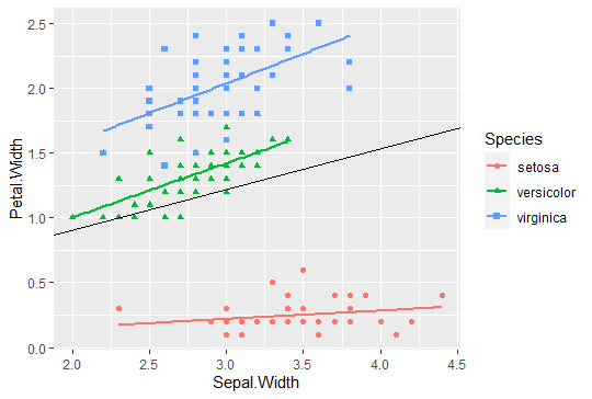
g<- ggplot(iris,aes(x=Sepal.Width, y=Petal.Width))+
geom_point(aes(color=Species,shape=Species))+
geom_smooth(method="lm",formula='y~x',aes(color=Species),se=FALSE)
geom_abline(intercept = r.fix[[1]] ,slope = r.fix[[2]],linetype=1)
plot(g)
混合モデルの変量効果の図示
Speciesの各種ごとにどれくらい変量効果が載っているかはranef()で得られます。
先の固定効果に変量効果を足し合わせたものが、各群の推定モデルになります。
ってことで、以下のようにすると図示できます。
なお以下では、geom_ablineに切片と傾きをベクトルで渡してます。
また、線は破線にして、色も分けてます。
さらに、見やすくするために背景の色もtheme()を使って変えてます。
r.lmer<- lmer(Petal.Width~Sepal.Width + (1+Sepal.Width|Species),iris)
summary(r.lmer)
r.fix <-fixef(r.lmer)
r.ran <-ranef(r.lmer)
#-------------------------------------
# $Species
#            (Intercept) Sepal.Width
# setosa     -0.31473162 -0.23095576
# versicolor  0.05920427  0.04344516
# virginica   0.25552735  0.18751059
#-------------------------------------

g<- ggplot(iris,aes(x=Sepal.Width, y=Petal.Width))+
  theme(panel.background = element_rect(fill = "gray"))+
  geom_point(aes(color=Species,shape=Species))+
  geom_smooth(method="lm",formula='y~x',aes(color=Species),se=FALSE)+
  geom_abline(intercept = r.fix[[1]] ,slope = r.fix[[2]],linetype=1)+
  geom_abline(intercept = (r.ran$Species$`(Intercept)`+r.fix[[1]]),
              slope = (r.ran$Species$Sepal.Width+r.fix[[2]]),
              linetype=2,
              size=1,
              color=c("red","green","blue")
              )
plot(g)
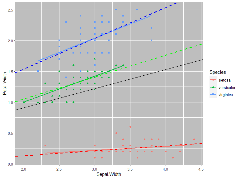
微妙に、それぞれ単独で回帰分析をかけた場合と異なっているのがわかります。