arxivの情報を使って特定分野の共著者ネットワークを書く

前書き

arxivから情報を収集して便利な情報がとれないかなと遊んでいる内容です。
今回やったことの手順は以下です。

1. 一定期間内に投稿された論文タイトル、アブスト、著者等を収集
2. 特定キーワードを含む論文を抽出
3. 抽出した論文と著者名の有向グラフを作成
4. 適当な閾値で投稿数が多い著者のみを抽出
5. 論文の数を辺の重みとする共著者グラフに変換
6. 連結かどうかで部分グラフに分割

適当なキーワードに関する研究分野内の大きな研究グループなどといったクラスタが見えないかなという奴です。
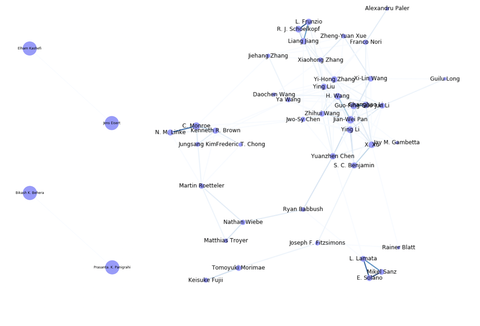
最終的に以下のグラフみたいな（論文数で条件付けられた）共著者ネットワークを抽出します。

arxivのquant-phの2015-2020年までの論文で、"quantum comput"をタイトル/アブストに含む論文を対象とし、該当論文が１５件以上ある著者のみを取り出したときの共著者ネットワークです。（辺の濃さが共著論文数・各クラスタごとで規格化）

(追記：著者名の表記揺れについて更新しデータを修正しました)

arxivから情報収集

Pythonで普通にスクレイピングします。（arxiv APIなるものもあったんですね）
arxivのAdvanced searchを直接叩いて拾っていきます。
1年毎に収集した情報をpandasのDataFrameにしてcsvとしてファイル保存します。

収集する情報は

• Cite : arxiv:XXXXXみたいな奴です。
• Title : 論文タイトル
• Abst : アブスト
• Authors : 著者リスト、リンクテキストになっている著者名と検索クエリに使われる文字列のタプルのリストで保存します。
• Fields : 分野情報です。Cross-listになっている場合は複数保存されます。
• DOI : DOIが追加されているものについては取得します。
• OrigDateY : 初回投稿年
• OrigDateM : 初回投稿月
• Date Info : その他の改版などの日付情報をテキストで保存します。

結局今回は使ってない情報もちらほら入っています。

※1年間の検索対象が10000件を超えるとarxivの仕様上動作しないということでコードを修正しました。件数を確認してオーバーする場合には月ごとに検索してデータ収集を行います。

from bs4 import BeautifulSoup
import requests
import re
import pandas as pd
import numpy as np
import math 

def month_string_to_number(string):
    m = {
        'jan': 1,
        'feb': 2,
        'mar': 3,
        'apr':4,
         'may':5,
         'jun':6,
         'jul':7,
         'aug':8,
         'sep':9,
         'oct':10,
         'nov':11,
         'dec':12
        }
    s = string.strip()[:3].lower()

    try:
        out = m[s]
        return out
    except:
        raise ValueError('Not a month')

# Search result のページから検索結果件数を取得
def get_number_of_searchresult(url):
    html_doc = requests.get(url).text
    soup = BeautifulSoup(html_doc, "html.parser") 
    tags = soup.find_all("h1",{"class":"title is-clearfix"})
    text = tags[0].text.strip()
    if "Showing" in text and "results" in text:
        stext = text.split(" ")
        datanum = int(stext[3].replace(',', ''))#検索結果の件数を取得
    else:
        datanum=math.nan
    return datanum

# Search resultsから情報取得しnp.ndarray化
def collect_info_from_advancedsearch(urlhead, datanum,key):

    titles=[]# データ保存用リスト
    absts=[]#Abst
    cites=[]# cite情報 (arxiv:XXXXXX)
    authors=[]# author
    dates=[]# 日付情報
    dates_orig_m =[]#初回投稿月
    dates_orig_y =[]#初回投稿年
    dois = []#doi
    fields=[]#cross-listを含む分野情報

    startnum=0
    while datanum > startnum:
        print(str(startnum)+"...", end="")
        url = urlhead+str(startnum)#advanced searchのURL 
        html_doc = requests.get(url).text
        soup = BeautifulSoup(html_doc, "html.parser") 

        # title情報
        tags1= soup.find_all("p", {"class": "title is-5 mathjax"}) 
        titles_tmp = [tag.text.strip() for tag in tags1]

        # abst情報
        tags2 = soup.find_all("span", {"class": "abstract-full has-text-grey-dark mathjax"})
        absts_tmp = [tag.text[:-7].strip() for tag in tags2 if "Less" in tag.text]

        # cite情報
        tags3 =soup.find_all("p", {"class": "list-title is-inline-block"})
        cites_tmp = [tag.select("a")[0].text for tag in tags3]

        # Date情報
        tags4 = soup.find_all("p",{"class":"is-size-7"})
        text = [tag.text.strip() for tag in tags4 if "originally announced" in tag.text ]
        dates_tmp = text
        dates_orig_y_tmp=[txt.split(" ")[-1][:-1] for txt in text]
        dates_orig_m_tmp=[month_string_to_number(txt.split(" ")[-2]) for txt in text]

        # DOI情報
        tags5 = soup.find_all("div",{"class":"is-marginless"})
        dois_tmp = [tag.text[tag.text.rfind("doi"):].split("\n")[1] for tag in tags5 if key in tag.text ]   

        # Author情報
        tags6= soup.find_all("p", {"class": "authors"}) 
        auths_tmp = []
        for tag in tags6:
            auths=tag.select("a")
            authlist=[(author.text,author.get("href")[33:]) for author in auths]
            auths_tmp.append(authlist)

        # Cross-list情報
        tags7= soup.find_all("div", {"class": "tags is-inline-block"})  # title#("span", {"class": "tag is-small is-link tooltip is-tooltip-top"})  # title
        fields_tmp=[tag.text.strip().split("\n") for tag in tags7]

        # 結果に追加
        titles.extend(titles_tmp)
        absts.extend(absts_tmp)
        cites.extend(cites_tmp)
        authors.extend(auths_tmp)
        dates.extend(dates_tmp)
        dates_orig_y.extend(dates_orig_y_tmp)
        dates_orig_m.extend(dates_orig_m_tmp)
        dois.extend(dois_tmp)
        fields.extend(fields_tmp)

        # 検索結果の次ページの開始番号更新
        startnum += sizenum

    nt = np.array(titles)
    na = np.array(absts)
    nauth = np.array(authors)
    ncite = np.array(cites)
    nd = np.array(dates)
    ndy = np.array(dates_orig_y)
    ndm = np.array(dates_orig_m)
    ndoi = np.array(dois)
    nfields=np.array(fields)
    npdataset = np.concatenate([[ncite],[nt],[na],[nauth],[nfields],[ndoi],[ndy],[ndm],[nd]],axis=0).T
    print(" collected data number : ", npdataset.shape[0])
    return npdataset

#検索クエリの検索対象分類の指定用辞書
dict_class={'cs': '&classification-computer_science=y',
 'econ': '&classification-economics=y',
 'eess': '&classification-eess=y',
 'math': '&classification-mathematics=y',
 'q-bio': '&classification-q_biology=y',
 'q-fin': '&classification-q_finance=y',
 'stat': '&classification-statistics=y',
 'all': '&classification-physics=y&classification-physics_archives=all',
 'astro-ph': '&classification-physics=y&classification-physics_archives=astro-ph',
 'cond-mat': '&classification-physics=y&classification-physics_archives=cond-mat',
 'gr-qc': '&classification-physics=y&classification-physics_archives=gr-qc',
 'hep-ex': '&classification-physics=y&classification-physics_archives=hep-ex',
 'hep-lat': '&classification-physics=y&classification-physics_archives=hep-lat',
 'hep-ph': '&classification-physics=y&classification-physics_archives=hep-ph',
 'hep-th': '&classification-physics=y&classification-physics_archives=hep-th',
 'math-ph': '&classification-physics=y&classification-physics_archives=math-ph',
 'nlin': '&classification-physics=y&classification-physics_archives=nlin',
 'nucl-ex': '&classification-physics=y&classification-physics_archives=nucl-ex',
 'nucl-th': '&classification-physics=y&classification-physics_archives=nucl-th',
 'physics': '&classification-physics=y&classification-physics_archives=physics',
 'quant-ph': '&classification-physics=y&classification-physics_archives=quant-ph'}

years = [y for y in range(2015,2020)]
key = "quant-ph"#検索対象の分野　dict_classのkeyを指定
output_fname="df_quant-ph" #出力ファイル名

url0="https://arxiv.org/search/advanced?advanced=&terms-0-operator=AND&terms-0-term=&terms-0-field=title"
url1="&classification-include_cross_list=include"
url_daterange="&date-year=&date-filter_by=date_range"
url2="&date-date_type=submitted_date&abstracts=show&size="
urlmid = "&order=-announced_date_first&start="

sizenum = 25
startnum=0
for year in years:
    m_divide = 1 # 検索期間の分割数
    mstart =1
    mstop = 1
    url_date = "&date-from_date="+str(year)+"-"+str(mstart).zfill(2)+"-01&date-to_date="+str(year+1)+"-"+str(mstop).zfill(2)+"-01"
    urlhead = url0+dict_class[key]+url1+url_daterange+url_date+url2
    urlmid = "&order=-announced_date_first&start="
    url = urlhead+str(sizenum)+urlmid+str(startnum)

    datanum=get_number_of_searchresult(url) #検索結果件数の取得
    print("Number of search results ("+str(year)+") : "+str(datanum))

    if datanum >=10000: #件数がLimitを超えた場合、1年間のデータ取得を月ごとに分割
        m_divide = 13
        for month_divide in range(2,12): #個別件数がLimit以下になる分割数の探索
            flag_numlimit = False
            for idx in range(month_divide):
                mstart = int(idx*12/month_divide+1)
                mstop = (int((idx+1)*12/month_divide)+1)%12
                if mstop !=1:
                    url_date = "&date-from_date="+str(year)+"-"+str(mstart).zfill(2)+"-01&date-to_date="+str(year)+"-"+str(mstop).zfill(2)+"-01"
                else:
                    url_date = "&date-from_date="+str(year)+"-"+str(mstart).zfill(2)+"-01&date-to_date="+str(year+1)+"-"+str(mstop).zfill(2)+"-01"

                urlhead = url0+dict_class[key]+url1+url_daterange+url_date+url2
                url = urlhead+str(sizenum)+urlmid+str(startnum)
                datanum=get_number_of_searchresult(url)#分割数ごとでのデータ件数取得
                if datanum >= 10000:
                    flag_numlimit = True
            if not flag_numlimit:
                m_divide = month_divide
                break
        if m_divide > 12:
            print("*** Number of search result is over the limit 10,000. Please refine your search. ***")

    sizenum=200
    npdataset = np.empty((0,9))
    for idx in range(m_divide):
        mstart = int(idx*12/m_divide+1)
        mstop = (int((idx+1)*12/m_divide)+1)%12
        if mstop !=1:
            url_date = "&date-from_date="+str(year)+"-"+str(mstart).zfill(2)+"-01&date-to_date="+str(year)+"-"+str(mstop).zfill(2)+"-01"
        else:
            url_date = "&date-from_date="+str(year)+"-"+str(mstart).zfill(2)+"-01&date-to_date="+str(year+1)+"-"+str(mstop).zfill(2)+"-01"

        urlhead = url0+dict_class[key]+url1+url_daterange+url_date+url2       
        url = urlhead+str(25)+urlmid+str(0)
        datanum=get_number_of_searchresult(url)

        print("Collect search results ..." + url_date + ", Number of search results : " + str(datanum))
        urlhead2 = urlhead+str(sizenum)+urlmid
        npdataset_tmp = collect_info_from_advancedsearch(urlhead2,datanum,key)
        npdataset = np.concatenate([npdataset, npdataset_tmp], axis=0)

    #1年分の情報をnumpy、pandas DataFrameに変換してcsvに保存
    dataset = pd.DataFrame(npdataset)
    dataset.columns =["Cite","Title","Abst","Authors","Fields","DOI", "OrigDateY","OrigDateM","Date Info"]
    dataset.to_csv(output_fname+str(year)+".csv")

特定キーワードを含む論文を抽出

年ごとに収集したcsvを読み込んで連結します。
連結したデータセットに対してタイトルとアブスト内にキーワードが含まれるものを抽出します。
今回はquantum computをキーワードにしています。

fname_head = "df_quant-ph"

fname = fname_head + str(2020)+".csv"
dataset = pd.read_csv(fname, index_col=0)

for year in range(2010,2020):
    fname = fname_head + str(year)+".csv"
    print(fname)
    dataset_tmp = pd.read_csv(fname, index_col=0)
    dataset = pd.concat([dataset,dataset_tmp])

dataset =dataset.reset_index()
dataset_r=dataset.query('title.str.contains("quantum comput")  or abst.str.contains("quantum comput")', engine='python')

ただこの形だと大文字小文字問題や、他の検索ワードの場合に適切に検索にかからないかと思ったので
nltkを使ったStemming処理も追加しました。ここを参考にしています。
Lemmatizationもとりあえず書いてますが今はコメントアウトしてます。

import re
import nltk
from nltk.corpus import stopwords
from nltk.stem.porter import PorterStemmer
from nltk.stem.wordnet import WordNetLemmatizer
from nltk.corpus import stopwords

def preprocess_text(text):
    text = re.sub('[^a-zA-Z]', ' ', text)#Remove punctuations
    text = text.lower()
    text=re.sub("</?.*?>"," <> ",text)#remove tags
    text=re.sub("(\\d|\\W)+"," ",text)# remove special characters and digits

    text = text.split()

    stop_words = set(stopwords.words("english"))
    ##Stemming
    #Lemmatisation
    ps=PorterStemmer()
    #lem = WordNetLemmatizer()
    text = [ps.stem(word) for word in text if not word in stop_words]
    text=" ".join(text)

    return text

ndata = (dataset['Title']+" "+ dataset['Abst']).values
ndata= np.array([preprocess_text(text) for text in ndata])
dataset['Keywords'] = ndata
dataset_r=dataset.query('Keywords.str.contains("quantum comput")', engine='python')

抽出した論文と著者名のグラフを作成

networkxを使って論文と著者の関係を辺とした有向グラフ（頂点は著者名と論文番号）を書きます。
author情報を読みづらい形式で入れてしまったのでちょっと変なことをしています。

追記：名前の一部がイニシャル化されたりされなかったりといった揺らぎについて、Family name以外？がイニシャル化されたクエリ文字列を使ってデータを取ります。（表記は最頻値一つを選んでいます。変えたい場合は別途辞書auth_dictをいじってください。）
ただしイニシャル化された文字列で検索するため過剰にまとめられてしまう著者名がありえます。
表記そのままで分類したい場合はコメントアウトされたauthnameを利用します。

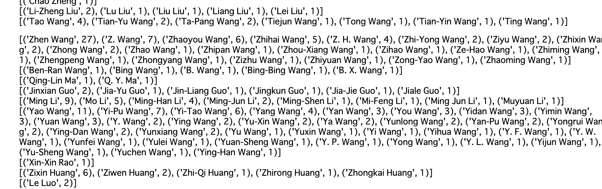
まとめられた著者名を確認するには

例えば以下のようなコードを実行すれば以下の画像のような出力が得られます。

authtext = " ".join(auths)
match = re.findall(r"(\()(.*?)\)",authtext)
for key in auth_dict.keys():
    l=[m[1].split(m[1][0])[1] for m in match if key in m[1]]
    c = collections.Counter(l)
    print(c.most_common())

import networkx as nx
import collections

auths= dataset_r['Authors'].values
datanum = auths.shape[0]

#著者名辞書の作成
auth_dict = {} 
for idx in range(datanum):
    match = re.findall(r"(\()(.*?)\)",auths[idx])
    for m in match:
        auth = m[1].split(m[1][-1])[-2]
        authname = m[1].split(m[1][0])[1]
        auth_dict[auth]=authname
#辞書の各項目を最頻値に変更
authtext = " ".join(auths)
match = re.findall(r"(\()(.*?)\)",authtext)
for key in auth_dict.keys():
    l=[m[1].split(m[1][0])[1] for m in match if key in m[1]]
    c = collections.Counter(l)
    auth_dict[key]=c.most_common()[0][0]

#グラフに情報追加
G=nx.DiGraph()
for idx in range(datanum):
    match = re.findall(r"(\()(.*?)\)",auths[idx])
    for m in match:
        auth = m[1].split(m[1][-1])[-2]
        #authname = m[1].split(m[1][0])[1]#表記のままでグラフ作成したい場合はこのauthnameで辺を追加する
        G.add_edges_from([(idx,auth_dict[auth])])

各著者に対して、論文数が少ない著者をグラフから除きます。（今回は15件以下を削除）
その結果、各論文に対して次数が0になったものを除きます。

thr=15
authorlist = [n  for n in G.nodes() if type(n) is str]
for auth in authorlist:
    deg=G.degree(auth)
    if deg <=thr:
        G.remove_node(auth)

for idx in range(datanum):
    deg=G.degree(idx)
    if deg <=0:
        G.remove_node(idx)

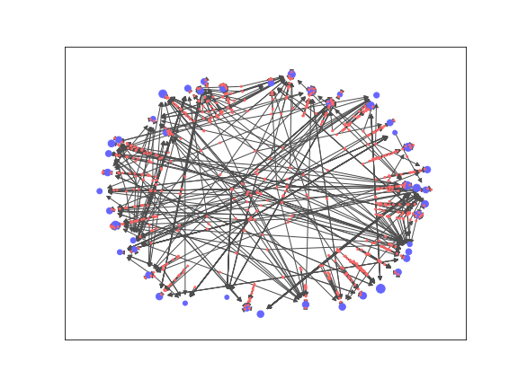
得られたグラフを描画します。
著者を青、論文を赤の頂点で描き、
PageRankを用いて重要な頂点はサイズを大きくしてみています。
こちらの記事を参考にしています。

def draw_graph(G, label = False):
    # pagerank の計算
    pr = nx.pagerank(G)
    pos = nx.spring_layout(G)

    fig = plt.figure(figsize=(8.0, 6.0))
    c=[(0.4,0.4,1) if type(n) is str else (1,0.4,0.4)  for n in G.nodes()]

    nx.draw_networkx_edges(G,pos, edge_color=(0.3,0.3,0.3))
    nx.draw_networkx_nodes(G,pos, node_color=c, node_size=[5000*v for v in pr.values()])

出力結果が以下です。
多くの論文が一人の著者のみを指すような状態になっています。

論文の数を辺の重みとする共著者グラフに変換

とりあえずの興味は共著者ネットワークだったので、論文の情報は辺の重みにしてしまいます。

import itertools

def convert_weightedGraph(graph):
    graph_new =nx.Graph()
    for node in graph.nodes:
        if type(node) is str:
            continue
        n_new = [e[1] for e in graph.edges if e[0]==node]
        for e_new in itertools.permutations(n_new, 2):

            flag_dup = False
            for e_check in graph_new.edges(data=True):
                if e_new[0] in e_check and e_new[1] in e_check:
                    e_check[2]['weight']+=1
                    flag_dup = True
            if not flag_dup:
                graph_new.add_edge(e_new[0],e_new[1],weight=1)
    return graph_new

wG=convert_weightedGraph(G)

得られたグラフを以下の関数で描画します。
ラベルが重なる場合は図のサイズやspring_layoutの引数kで調整できます。(参考)

def draw_weightedG(G):
    fig = plt.figure(figsize=(8.0, 6.0))
    pr = nx.pagerank(G)
    pos = nx.fruchterman_reingold_layout(G,k=k0/math.sqrt(G.order()))
    #pos = nx.spring_layout(G,k=15/math.sqrt(G.order())) 
    #適当なlayoutを使う。kの値でノード間距離を微調整  


    x_values, y_values = zip(*pos.values())
    x_max = max(x_values)
    x_min = min(x_values)
    x_margin = (x_max - x_min) * 0.25
    plt.xlim(x_min - x_margin, x_max + x_margin) #ラベル文字が切れないようにマージン確保

    node_sizes=[5000*v for v in pr.values()]
    edge_colors = [e[2]['weight'] for e in G.edges(data=True)] #辺の重みで色付け
    nodes = nx.draw_networkx_nodes(G, pos, node_size=node_sizes, node_color='#9999ff')
    edges = nx.draw_networkx_edges(G, pos, node_size=node_sizes, arrowstyle='->',
                                   arrowsize=10, edge_color=edge_colors,
                                   edge_cmap=plt.cm.Blues, width=2)
    nx.draw_networkx_labels(G,pos)

    ax = plt.gca()
    ax.set_axis_off()

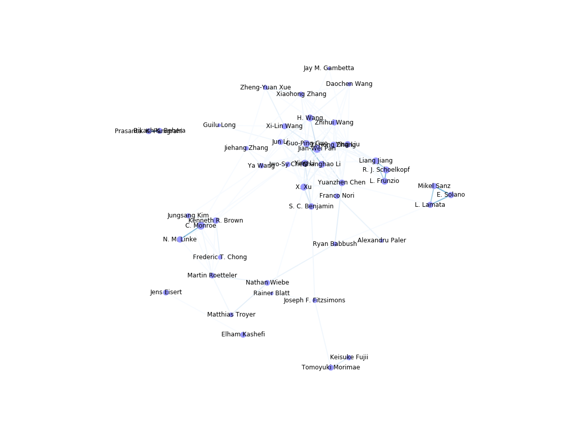
得られたグラフの描画結果から、非連結な部分グラフがあることがわかります。

連結かどうかで部分グラフに分割

グラフの各ノードを起点として連結な部分グラフを作っていきます。
ぱっと見で使えそうな道具がなかったのでベタ書きしてます。

def add_edges_to_wsubgraph(subg, edge_new,node,edges_all):
    subg.add_edges_from([edge_new])

    if node == edge_new[1]:
        node_new = edge_new[0]
    else:
        node_new = edge_new[1]

    edges_new = [e for e in edges_all if node_new in e and e not in subg.edges(data=True)]
    for edge in edges_new:
        if edge not in subg.edges(data=True):
            add_edges_to_wsubgraph(subg,edge,node_new,edges_all)

def separate_wG_by_connectivity(G):
    nodes_all =[n for n in G.nodes()]
    edges_all = [e for e in G.edges(data=True)]
    subgraphs = []

    for node in nodes_all:
        usedflag = any([node in g.nodes for g in subgraphs])
        if usedflag:
            continue 

        subg = nx.Graph()
        subg.add_node(node)
        edges_new = [e for e in edges_all if node in e]
        for edge in edges_new:
            if edge not in subg.edges(data=True):
                add_edges_to_wsubgraph(subg,edge,node,edges_all)
        subgraphs.append(subg)

    return subgraphs

subgraphs = separate_wG_by_connectivity(wG)

ここで得られた部分グラフをそれぞれ描画すると
以下のような３つのグラフが得られます。(手動で１枚の画像にしています)

cnt=0
for subg in subgraphs:#部分グラフを描画、画像保存
    draw_weightedG(subg)
    plt.savefig("subgraph_"+str(cnt)+".png")
    plt.cla()
    cnt+=1

まとめ

arxivからのデータ取得からはじめ、特定キーワードに関する共著者ネットワーク的な物を書いてみました。
結果には比較的きれいなものを持ってきましたが、検索キーワードやしきい値の設定によっては大きいクラスタだけが残る状況もありました。
そうした場合には、辺の重みになっている共著論文数を適当なしきい値で切っていくともうちょっと細かい様子が取れるかもしれないです。
後は論文の引用被引用関係などが取れると面白そうだなとは思いますが、手軽な情報収集元が思いつかなかったので何か教えてもらえたら嬉しいです。