Pythonで学ぶ音信号処理(ディストーション＋コンプレッサー処理)

---

Pythonで「ドの音」を歪ませて圧縮する：ディストーション＋コンプレッサー処理の可視化と再生

はじめに

本記事では、Pythonを用いて「ドの音（C4, 261.63 Hz）」のサイン波を生成し、それに対して以下の2つの音響エフェクト処理を施します：

• ディストーション（非線形歪み）
• コンプレッサー（ダイナミックレンジ圧縮）

さらに、波形の可視化と各信号の周期・周波数の解析、Google Colabでの音再生まで一貫して行います。

---

使用するPython技術

• NumPy（数値計算）
• Matplotlib（波形可視化）
• IPython.display.Audio（音再生）
• サイン波生成、ゼロクロス法による周波数推定、非線形マッピング

---

import numpy as np
import matplotlib.pyplot as plt
from IPython.display import Audio, display

# --- 基本設定 / Basic Parameters ---
amplitude = 1.0
new_frequency = 261.63  # 「ド」の音 / Middle C (C4)
sample_rate = 44100           # サンプリングレート
duration = 2                  # 音の長さ（秒）

# --- 時間軸と入力信号 / Time axis and input sine wave ---
time_full = np.linspace(0, duration, int(sample_rate * duration))
sine_wave_full = amplitude * np.sin(2 * np.pi * new_frequency * time_full)

# --- ディストーション関数（非線形歪み）/ Distortion Function ---
def distortion_mapping(x):
    return 2 / (1 + np.exp(-5 * x)) - 1

# --- コンプレッサ関数（ダイナミックレンジ圧縮）/ Compressor Function ---
def compressor_mapping(x, T=0.5, R=4.0, W=0.2):
    y = np.zeros_like(x)
    for i, val in enumerate(x):
        abs_x = abs(val)
        if abs_x < T - W/2:
            y[i] = val
        elif abs_x < T + W/2:
            gain = (1 - 1/R) * (abs_x - T)**2 / (2 * W)
            y[i] = np.sign(val) * (T + gain)
        else:
            y[i] = np.sign(val) * (T + (abs_x - T) / R)
    return y

# --- 処理ステップ / Processing Steps ---
distorted_signal = distortion_mapping(sine_wave_full)
compressed_signal = compressor_mapping(distorted_signal)

# --- 各信号の周期の推定 / Estimate Period of Each Signal ---
def estimate_period(signal, fs):
    # ゼロクロス（正→負）を検出し、その間隔で周期を推定 / Use zero-crossing (positive-going) for estimation
    zero_crossings = np.where((signal[:-1] < 0) & (signal[1:] >= 0))[0]
    if len(zero_crossings) < 2:
        return None, None
    periods = np.diff(zero_crossings) / fs  # 秒単位
    avg_period = np.mean(periods)
    freq = 1 / avg_period
    return avg_period, freq

# 周期と周波数を計算 / Calculate for all signals
period_input, freq_input = estimate_period(sine_wave_full, sample_rate)
period_dist, freq_dist = estimate_period(distorted_signal, sample_rate)
period_comp, freq_comp = estimate_period(compressed_signal, sample_rate)

# --- 周波数・周期表示 / Print periods and frequencies ---
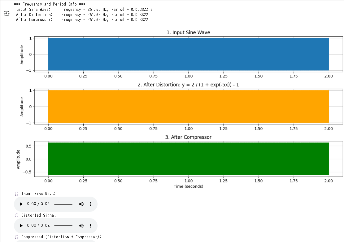
print("=== Frequency and Period Info ===")
print(f" Input Sine Wave:     Frequency ≈ {freq_input:.2f} Hz, Period ≈ {period_input:.6f} s")
print(f" After Distortion:    Frequency ≈ {freq_dist:.2f} Hz, Period ≈ {period_dist:.6f} s")
print(f" After Compressor:    Frequency ≈ {freq_comp:.2f} Hz, Period ≈ {period_comp:.6f} s\n")

# --- 可視化 / Plotting ---
plt.figure(figsize=(12, 6))
plt.subplot(3, 1, 1)
plt.plot(time_full, sine_wave_full)
plt.title("1. Input Sine Wave")
plt.ylabel("Amplitude")
plt.grid(True)

plt.subplot(3, 1, 2)
plt.plot(time_full, distorted_signal, color='orange')
plt.title("2. After Distortion: y = 2 / (1 + exp(-5x)) - 1")
plt.ylabel("Amplitude")
plt.grid(True)

plt.subplot(3, 1, 3)
plt.plot(time_full, compressed_signal, color='green')
plt.title("3. After Compressor")
plt.xlabel("Time (seconds)")
plt.ylabel("Amplitude")
plt.grid(True)

plt.tight_layout()
plt.show()

# --- 音の再生 / Play Audio ---
print("🎧 Input Sine Wave:")
display(Audio(sine_wave_full, rate=sample_rate))

print("🎧 Distorted Signal:")
display(Audio(distorted_signal, rate=sample_rate))

print("🎧 Compressed (Distortion + Compressor):")
display(Audio(compressed_signal, rate=sample_rate))

結果

説明

入力信号：ドの音のサイン波

サンプリング周波数44.1kHz、振幅1.0、周波数261.63Hz（ドの音）で2秒間のサイン波を生成します。

new_frequency = 261.63  # 「ド」の音 / Middle C (C4)
sine_wave_full = amplitude * np.sin(2 * np.pi * new_frequency * time_full)

---

ディストーション処理（非線形変換）

以下の非線形マッピング関数を使用して、入力波形を歪ませます：

[
y = \frac{2}{1 + \exp(-5x)} - 1
]

この式はスケーリングされたシグモイド関数で、-1〜+1の範囲に収めつつ、入力に非線形な歪みを加えます。

def distortion_mapping(x):
    return 2 / (1 + np.exp(-5 * x)) - 1

---

コンプレッサー処理（ダイナミックレンジ圧縮）

以下のような条件に基づき、ソフトニー付きのコンプレッサーを適用します：

• ( x < T - W/2 )：そのまま通す
• ( T - W/2 \leq x < T + W/2 )：滑らかに圧縮開始
• ( x \geq T + W/2 )：圧縮比に従って抑制

def compressor_mapping(x, T=0.5, R=4.0, W=0.2):
    ...

---

波形の可視化

以下は、ディストーション関数とコンプレッサ関数の入力出力特性を可視化するPythonコードです。プロットにより、それぞれの関数が信号にどのような変換を施すかがわかります。コメントは日本語と英語で記述しています。

import numpy as np
import matplotlib.pyplot as plt

# --- ディストーション関数 / Distortion Mapping Function ---
def distortion_mapping(x):
    return 2 / (1 + np.exp(-5 * x)) - 1

# --- コンプレッサ関数 / Compressor Mapping Function ---
def compressor_mapping(x, T=0.5, R=2.0, W=0.2):
    y = np.zeros_like(x)
    for i, val in enumerate(x):
        abs_x = abs(val)
        if abs_x < T - W/2:
            y[i] = val  # リニア領域 / Linear region
        elif abs_x < T + W/2:
            gain = (1 - 1/R) * (abs_x - T)**2 / (2 * W)
            y[i] = np.sign(val) * (T + gain)  # ソフトニー領域 / Soft knee region
        else:
            y[i] = np.sign(val) * (T + (abs_x - T) / R)  # 圧縮領域 / Compression region
    return y

# 入力値の範囲 / Input range
x = np.linspace(-1.5, 1.5, 1000)

# 出力値の計算 / Compute output values
y_dist = distortion_mapping(x)
y_comp = compressor_mapping(x)

# --- プロット / Plot ---
plt.figure(figsize=(10, 5))

# Distortion
plt.subplot(1, 2, 1)
plt.plot(x, y_dist, label='Distortion')
plt.title("Distortion Mapping")
plt.xlabel("Input")
plt.ylabel("Output")
plt.grid(True)
plt.legend()

# Compressor
plt.subplot(1, 2, 2)
plt.plot(x, y_comp, label='Compressor', color='orange')
plt.title("Compressor Mapping")
plt.xlabel("Input")
plt.ylabel("Output")
plt.grid(True)
plt.legend()

plt.tight_layout()
plt.show()

---

周期と周波数の解析（ゼロクロス法）

以下の関数を用いて、各波形の**周期（Period）と周波数（Frequency）**を自動推定します：

def estimate_period(signal, fs):
    zero_crossings = np.where((signal[:-1] < 0) & (signal[1:] >= 0))[0]
    ...

出力例（ドの音）：

=== Frequency and Period Info ===
 Input Sine Wave:     Frequency ≈ 261.63 Hz, Period ≈ 0.003821 s
 After Distortion:    Frequency ≈ 261.63 Hz, Period ≈ 0.003821 s
 After Compressor:    Frequency ≈ 261.63 Hz, Period ≈ 0.003821 s

周波数は処理しても変わらないことが確認できます。変わるのは波形の形（＝倍音構成）です。

---

音の再生（Google Colab）

Colab環境では IPython.display.Audio を用いて各処理段階の音を試聴できます：

display(Audio(sine_wave_full, rate=sample_rate))      # 入力波
display(Audio(distorted_signal, rate=sample_rate))     # 歪み
display(Audio(compressed_signal, rate=sample_rate))    # 歪み＋圧縮

---

---

まとめ

処理段階	主な効果	波形変化	周波数変化
入力サイン波	原音（純音）	正弦波	261.63 Hz
ディストーション	倍音を付加	非対称	変わらず
コンプレッサー	音量を平滑化	ダイナミクス抑制	変わらず

---

参考図書

Pythonではじめる音のプログラミング －コンピュータミュージックの信号処理－
https://www.amazon.co.jp/gp/product/B0BFZNHS2R?ie=UTF8&psc=1&linkCode=sl1&tag=hcrane-22&linkId=cf740dda8a119a71a777903335c8f8d0&language=ja_JP&ref_=as_li_ss_tl