SymPy・LaTeX・HTML・数式表示を組み合わせてPythonコードで出力

はじめに

本記事では、SymPy・LaTeX・HTML・数式表示を組み合わせて、三平方の定理（ピタゴラスの定理）を視覚的にわかりやすく解説するPythonコードをご紹介します。
Jupyter Notebook や Google Colab 上で使えるこのコードは、数式を美しくレンダリングしながら、理論と実例を直感的に理解できる構成になっています。

教材づくりや学習メモ、教育用途にも活用できるので、ぜひご活用ください。

Pythonコード

from sympy import symbols, Eq, latex
from IPython.display import display, HTML, Math
import sympy as sp
import matplotlib.pyplot as plt

# 変数の定義（Define variables）
a, b, c = symbols('a b c')
pythagorean_theorem = Eq(c**2, a**2 + b**2)
latex_eq = latex(pythagorean_theorem)

# タイトルのHTML（Title section）
header_html = """
<div style="font-size:28px; font-family:'Yu Mincho', 'Hiragino Mincho ProN', serif; font-weight:bold;">
三平方の定理（ピタゴラスの定理）
</div>
"""

# 本文のHTML（Body section with Japanese + LaTeX inline）
body_html = """
<div style="font-size:18px; font-family:'Yu Gothic', 'Hiragino Kaku Gothic ProN', sans-serif;">
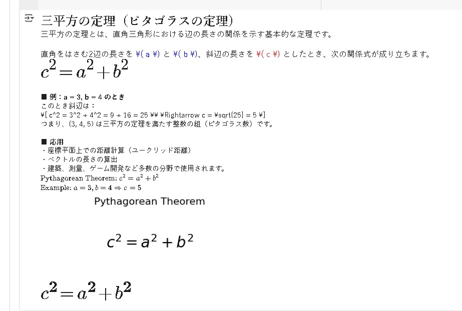
三平方の定理とは、直角三角形における辺の長さの関係を示す基本的な定理です。<br><br>
直角をはさむ2辺の長さを <span style="color:blue;">\\( a \\)</span> と <span style="color:blue;">\\( b \\)</span>、斜辺の長さを <span style="color:red;">\\( c \\)</span> としたとき、次の関係式が成り立ちます。
</div>
"""

# 数式（Equation rendering with size）
equation_latex = f"\\displaystyle \\Huge {latex_eq}"

# 応用・例のHTML（Applications and example）
example_html = """
<div style="font-size:16px; font-family:'Yu Gothic', sans-serif;">
<br>
<b>■ 例：a = 3, b = 4 のとき</b><br>
このとき斜辺は：<br>
\\[
c^2 = 3^2 + 4^2 = 9 + 16 = 25 \\\\
\\Rightarrow c = \\sqrt{25} = 5
\\]<br>
つまり、(3, 4, 5) は三平方の定理を満たす整数の組（ピタゴラス数）です。<br><br>

<b>■ 応用</b><br>
・座標平面上での距離計算（ユークリッド距離）<br>
・ベクトルの長さの算出<br>
・建築、測量、ゲーム開発など多数の分野で使用されます。<br>
</div>
"""

# 表示（Render all）
display(HTML(header_html))
display(HTML(body_html))
display(Math(equation_latex))
display(HTML(example_html))

# シンボルの定義（再度）
a, b, c = sp.symbols('a b c')

# 三平方の定理
pythagoras_eq = sp.Eq(c**2, a**2 + b**2)

# LaTeX表示（サイズ指定なし）
display(Math(r"\text{Pythagorean Theorem: } c^2 = a^2 + b^2"))

# 例：a = 3, b = 4 の場合のcを計算
solution = sp.solve(pythagoras_eq.subs({a: 3, b: 4}), c)
display(Math(r"\text{Example: } a=3, b=4 \Rightarrow c = " + sp.latex(solution[1])))

# Matplotlibで数式を表示
plt.figure(figsize=(6, 2))
plt.text(0.5, 0.5, r"$c^2 = a^2 + b^2$", fontsize=24, ha='center', va='center')
plt.axis('off')
plt.title("Pythagorean Theorem", fontsize=16)
plt.show()

# IPython DisplayでLaTeX数式を表示（サイズ調整）
display(Math(r"\displaystyle \textbf{\Huge $c^2 = a^2 + b^2$}"))

結果