初代ガンダムとジークアクスからはじめる5倍ゲイン制御工学

参考リンクまとめ

Pythonコード

# Program Name: energy_gain_with_feedback_and_cutoff.py
# Creation Date: 20250418
# Overview:
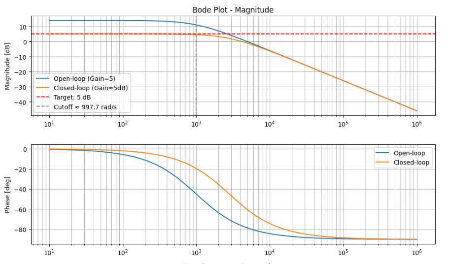
# 「5倍のエネルギーゲインがある」一次遅れ系のボード線図、ステップ応答、カットオフ周波数（-3dB）を表示する
# 『機動戦士ガンダム』第1話「ガンダム大地に立つ!!」にて、
# アムロ・レイがマニュアルとメーターを見ながら驚きと共に発したセリフ
# 「すごい、5倍以上のエネルギーゲインがある！」をもとに、
# それを制御工学の「ゲイン」としてモデル化。
# 「5倍のエネルギーゲインがある」一次遅れ系のボード線図、ステップ応答、カットオフ周波数（-3dB）を表示する
# さらに、5dBの増幅となるようなフィードバック係数βを導入した閉ループ系の解析も追加する
# This program models a first-order lag system with gain of 5 and adds feedback to achieve 5dB amplification.
# It visualizes Bode plots, step responses, and cutoff frequency for both open-loop and closed-loop systems.

import numpy as np
import matplotlib.pyplot as plt
from scipy import signal

# --- システムパラメータ / System parameters ---
K = 5.0        # 開ループゲイン / Open-loop gain
tau = 0.001    # 時定数 / Time constant [s]

# --- フィードバックによる5dBゲイン調整 / Feedback for 5 dB total gain ---
target_dB = 5                                      # 目標ゲイン / Target gain [dB]
G_target = 10**(target_dB / 20)                    # 線形ゲイン / Linear gain
beta = (K - G_target) / (K * G_target)             # β = (K - G_target) / (K * G_target)
K_cl = K / (1 + beta * K)                          # 確認用: 閉ループDCゲイン

# --- 開ループ伝達関数 / Open-loop transfer function ---
num_ol = [K]
den_ol = [tau, 1]
sys_ol = signal.TransferFunction(num_ol, den_ol)

# --- 閉ループ伝達関数 / Closed-loop transfer function ---
num_cl = [K]
den_cl = [tau, 1 + beta * K]
sys_cl = signal.TransferFunction(num_cl, den_cl)

# --- ボード線図 / Bode plot ---
w = np.logspace(1, 6, 3000)
w, mag_ol, phase_ol = signal.bode(sys_ol, w=w)
_, mag_cl, phase_cl = signal.bode(sys_cl, w=w)

# --- カットオフ周波数（開ループ）/ Cutoff frequency for open-loop ---
gain_ol_dB = 20 * np.log10(K)
cutoff_dB = gain_ol_dB - 3
cutoff_index = np.where(mag_ol <= cutoff_dB)[0]
cutoff_freq = w[cutoff_index[0]] if len(cutoff_index) > 0 else None

# --- ステップ応答 / Step response ---
t, y_ol = signal.step(sys_ol)
_, y_cl = signal.step(sys_cl)

# --- プロット開始 / Plotting ---
plt.figure(figsize=(10, 9))

# --- Bode Magnitude ---
plt.subplot(3, 1, 1)
plt.semilogx(w, mag_ol, label="Open-loop (Gain=5)")
plt.semilogx(w, mag_cl, label="Closed-loop (Gain=5dB)")
plt.axhline(20 * np.log10(G_target), color='red', linestyle='--', label="Target: 5 dB")
if cutoff_freq:
    plt.axvline(cutoff_freq, color='gray', linestyle='--', label=f"Cutoff ≈ {cutoff_freq:.1f} rad/s")
plt.title("Bode Plot - Magnitude")
plt.ylabel("Magnitude [dB]")
plt.grid(True, which="both")
plt.legend()

# --- Bode Phase ---
plt.subplot(3, 1, 2)
plt.semilogx(w, phase_ol, label="Open-loop")
plt.semilogx(w, phase_cl, label="Closed-loop")
plt.ylabel("Phase [deg]")
plt.grid(True, which="both")
plt.legend()

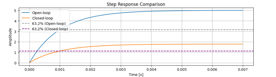
# --- Step Response ---
plt.subplot(3, 1, 3)
plt.plot(t, y_ol, label="Open-loop")
plt.plot(t, y_cl, label="Closed-loop")
plt.axhline(K * 0.632, color='gray', linestyle='--', label="63.2% (Open-loop)")
plt.axhline(K_cl * 0.632, color='purple', linestyle='--', label="63.2% (Closed-loop)")
plt.xlabel("Time [s]")
plt.ylabel("Amplitude")
plt.title("Step Response Comparison")
plt.grid(True)
plt.legend()

plt.tight_layout()
plt.show()
# --- パラメータ定義 / Define system parameters ---
K = 5.0                    # 開ループゲイン / Open-loop gain
tau = 0.001                # 時定数 / Time constant [s]
target_dB = 5              # ターゲットゲイン（dB）/ Target closed-loop gain [dB]
G_target = 10**(target_dB / 20)  # 線形ゲイン = 1.778 / Linear gain equivalent to 5 dB
beta = (K - G_target) / (K * G_target)  # 負帰還係数 / Feedback coefficient
K_cl = K / (1 + beta * K)  # 閉ループゲイン / Closed-loop gain

# --- 伝達関数表現 / Transfer Function Form ---
num_cl = [K]
den_cl = [tau, 1 + beta * K]
system_tf = signal.TransferFunction(num_cl, den_cl)

# --- 状態空間表現への変換 / Convert to state-space representation ---
# dx/dt = Ax + Bu, y = Cx + Du
A = np.array([[-(1 + beta * K) / tau]])  # 状態行列 / State matrix
B = np.array([[K / tau]])                # 入力行列 / Input matrix
C = np.array([[1]])                      # 出力行列 / Output matrix
D = np.array([[0]])                      # ダイレクト伝達 / Direct term

system_ss = signal.StateSpace(A, B, C, D)

# --- ステップ応答 / Step responses ---
t_tf, y_tf = signal.step(system_tf)
t_ss, y_ss = signal.step(system_ss)

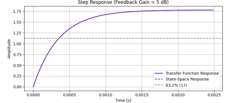
# --- 応答の描画 / Plot responses ---
plt.figure(figsize=(8, 4))
plt.plot(t_tf, y_tf, label="Transfer Function Response", color='blue')
plt.plot(t_ss, y_ss, '--', label="State-Space Response", color='purple')
plt.axhline(K_cl * 0.632, color='gray', linestyle='--', label="63.2% (1τ)")
plt.title("Step Response (Feedback Gain = 5 dB)")
plt.xlabel("Time [s]")
plt.ylabel("Amplitude")
plt.grid(True)
plt.legend()
plt.tight_layout()
plt.show()

結果