Pythonで学ぶシンセサイザー入門

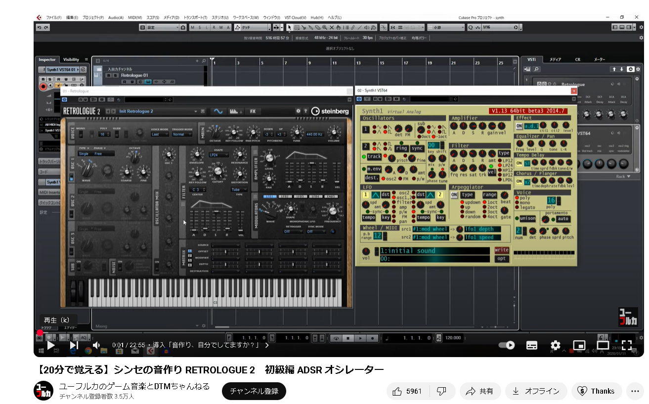
はじめに

音作りにおいて、「どんな波形を使うか」と同じくらい重要なのが、音の時間的な変化です。
音はただ鳴るだけでなく、「どのように立ち上がり」「どのように減衰し」「どれだけ続き」「どう消えていくか」といった**ダイナミクス（変化）**を持っています。

このページでは、

ADSRエンベロープによる音量変化の仕組み

5種類の基本波形（サイン波・矩形波・のこぎり波・三角波・ノイズ）
をPythonで視覚的に比較しながら、音の基本構造を理解します。

参考リンクまとめ

エンベロープ（Envelope）とは？

エンベロープとは、音の時間的な変化を制御するパラメータで、音の「鳴り始め〜消えるまで」の音量（Amplitude）や音色の変化を表現します。

特に代表的なのが ADSRエンベロープ です：

項目	説明
A (Attack)	鳴り始めから最大音量になるまでの時間（例：ピアノなら一瞬、バイオリンならゆっくり）
D (Decay)	最大音量から減衰して、一定音量に落ち着くまでの時間
S (Sustain)	鍵盤を押し続けている間、音が保たれる音量（音量の高さ）
R (Release)	鍵盤を離してから音が完全に消えるまでの時間

音の立ち上がり方、減衰、持続、消え方を「エンベロープ」でコントロールできます。

---

アンプ（アンプリファイヤー）とADSR

アンプリファイヤー（amplifier）は音の信号を増幅する回路ですが、シンセサイザーではしばしばエンベロープで制御されるボリューム調整回路として使われます。

具体的には：

• ADSRエンベロープの出力を使って、アンプの音量（ゲイン）を制御
• これにより、鍵盤を押した時に「どんなふうに音が出るか（パンッ、フワッなど）」が決まります

---

オシレーター（Oscillator）

オシレーターは、音の元となる波形を発生させる装置です。

• 周波数（Hz）で音の高さ（音程）
• 波形の種類で音のキャラクター（音色）

---

波の種類とその音色の特徴

波形	特徴	音の例
サイン波 (Sine wave)	純粋な音。倍音なし。	チューニング音、電子音
矩形波 (Square wave)	奇数次の倍音を持つ。ブリブリした音	ファミコン、ゲーム音
のこぎり波 (Sawtooth wave)	奇数・偶数両方の倍音。明るく鋭い音	シンセのストリングス
三角波 (Triangle wave)	サイン波に近いが、奇数次倍音あり	ソフトで控えめな音
ノイズ (Noise)	ランダム成分。ピチピチ・ザザッとした音	ドラム、効果音、風音

---

ADSRエンベロープによる音量変化と5種類の波形の視覚的比較

---

import numpy as np
import matplotlib.pyplot as plt

# サンプリング周波数と時間軸設定 / Sampling frequency and time axis
fs = 44100  # Hz
duration = 1.0  # 秒 / seconds
t = np.linspace(0, duration, int(fs * duration), endpoint=False)

# ADSRパラメータ設定 / ADSR envelope parameters
attack_time = 0.1    # Attack
decay_time = 0.1     # Decay
sustain_level = 0.7  # Sustain level
release_time = 0.2   # Release
sustain_time = duration - (attack_time + decay_time + release_time)

# 各セクションのサンプル数 / Sample count for each section
a_samples = int(fs * attack_time)
d_samples = int(fs * decay_time)
s_samples = int(fs * sustain_time)
r_samples = int(fs * release_time)

# ADSR エンベロープ生成 / Generate ADSR envelope
attack = np.linspace(0, 1, a_samples)
decay = np.linspace(1, sustain_level, d_samples)
sustain = np.ones(s_samples) * sustain_level
release = np.linspace(sustain_level, 0, r_samples)

adsr = np.concatenate((attack, decay, sustain, release))  # 完全なエンベロープ

# 波形生成関数 / Waveform generation functions
def sine_wave(freq, t): return np.sin(2 * np.pi * freq * t)
def square_wave(freq, t): return np.sign(np.sin(2 * np.pi * freq * t))
def sawtooth_wave(freq, t): return 2 * (t * freq - np.floor(0.5 + t * freq))
def triangle_wave(freq, t): return 2 * np.abs(sawtooth_wave(freq, t)) - 1
def noise_wave(t): return np.random.uniform(-1, 1, len(t))

# 波形データ生成 / Generate waveform data
freq = 440  # A4
waves = {
    "Sine": sine_wave(freq, t),
    "Square": square_wave(freq, t),
    "Sawtooth": sawtooth_wave(freq, t),
    "Triangle": triangle_wave(freq, t),
    "Noise": noise_wave(t)
}

# --- プロット開始 / Start plotting ---
plt.figure(figsize=(12, 16))

# ① 上：ADSRエンベロープ
plt.subplot(7, 1, 1)
plt.plot(t[:len(adsr)], adsr)
plt.title("ADSR Envelope")
plt.xlabel("Time [s]")
plt.ylabel("Amplitude")
plt.grid(True)

# ② 中：5種類の基本波形（別々にプロット）
for i, (name, wave) in enumerate(waves.items()):
    plt.subplot(7, 1, i + 2)
    plt.plot(t[:1000], wave[:1000])  # 最初の1000サンプルのみ表示
    plt.title(f"{name} Wave")
    plt.xlabel("Time [s]")
    plt.ylabel("Amplitude")
    plt.grid(True)

# ③ 下：ADSR × のこぎり波（例）
plt.subplot(7, 1, 7)
t_env = t[:len(adsr)]
saw_env_wave = sawtooth_wave(freq, t_env) * adsr
plt.plot(t_env, saw_env_wave)
plt.title("Sawtooth Wave with ADSR Envelope")
plt.xlabel("Time [s]")
plt.ylabel("Amplitude")
plt.grid(True)

plt.tight_layout()
plt.show()

---

デジタルフィルタのボード線図とSI単位接頭辞の表示

import numpy as np
import matplotlib.pyplot as plt
from scipy import signal

# ==== 基本パラメータ / Basic parameters ====
fs = 48000  # サンプリング周波数 [Hz] / Sampling frequency
fc = 2000   # カットオフ周波数 [Hz] / Cutoff frequency
order = 2   # フィルタ次数 / Filter order

# ==== フィルタ設計 / Filter design ====
# ローパスフィルタ / Low-pass
b_lpf, a_lpf = signal.butter(order, fc / (fs / 2), btype='low')
# ハイパスフィルタ / High-pass
b_hpf, a_hpf = signal.butter(order, fc / (fs / 2), btype='high')
# バンドパスフィルタ / Band-pass
b_bpf, a_bpf = signal.butter(order, [fc*0.5 / (fs / 2), fc*1.5 / (fs / 2)], btype='band')

# ==== 周波数応答（デジタル用）/ Frequency response for digital filters ====
w, h_lpf = signal.freqz(b_lpf, a_lpf, worN=1024, fs=fs)
_, h_hpf = signal.freqz(b_hpf, a_hpf, worN=1024, fs=fs)
_, h_bpf = signal.freqz(b_bpf, a_bpf, worN=1024, fs=fs)

# ==== 振幅応答プロット / Magnitude response plot ====
plt.figure(figsize=(10, 6))
plt.semilogx(w, 20 * np.log10(np.abs(h_lpf)), label='Low-pass Filter')
plt.semilogx(w, 20 * np.log10(np.abs(h_hpf)), label='High-pass Filter')
plt.semilogx(w, 20 * np.log10(np.abs(h_bpf)), label='Band-pass Filter')
plt.axvline(fc, color='gray', linestyle='--', label=f'Cutoff {fc} Hz')
plt.title("Bode Plot (Magnitude)")
plt.xlabel("Frequency [Hz]")
plt.ylabel("Gain [dB]")
plt.grid(which='both', linestyle='--', linewidth=0.5)
plt.legend()
plt.tight_layout()
plt.show()

# ==== 位相応答プロット / Phase response plot ====
plt.figure(figsize=(10, 6))
plt.semilogx(w, np.angle(h_lpf, deg=True), label='Low-pass Filter')
plt.semilogx(w, np.angle(h_hpf, deg=True), label='High-pass Filter')
plt.semilogx(w, np.angle(h_bpf, deg=True), label='Band-pass Filter')
plt.axvline(fc, color='gray', linestyle='--', label=f'Cutoff {fc} Hz')
plt.title("Bode Plot (Phase)")
plt.xlabel("Frequency [Hz]")
plt.ylabel("Phase [degrees]")
plt.grid(which='both', linestyle='--', linewidth=0.5)
plt.legend()
plt.tight_layout()
plt.show()

# ==== SI単位接頭辞リストを表示 / Print SI unit prefixes ====
si_prefixes = {
    "p": 1e-12,
    "n": 1e-9,
    "µ": 1e-6,
    "m": 1e-3,
    "": 1,
    "k": 1e3,
    "M": 1e6,
    "G": 1e9,
    "T": 1e12
}

print(" SI単位接頭辞（SI Unit Prefixes）")
for prefix, value in si_prefixes.items():
    print(f"{prefix}: {value:.0e}")