NTTドコモ R&D Advent Calendar 2020 の9日目の記事となります。
NTTドコモ1年目の島田です。普段はグロースハックチームでデータ分析業務をしています。
今回は、時系列予測ツールProphetと、ハイパーパラメータ自動最適化フレームワークOptunaを組み合わせたら、どのくらい精度があがるのかを試してみました。
そもそも
時系列予測となると、特に統計モデルの知識やドメイン知識が必要になります。
古典的なARIMAや状態空間モデルを使うのであれば統計の知識が求められますし
機械学習で予測するにしても、「季節性を表現する特徴量構築」のフェーズがあり、
データを観察し、ドメイン知識を利用しながら特徴量を慎重に設計する必要があります。
また、時系列データの場合、データ量が少ないことが多々あります。
日次データになると、1年分だとしても365点しかデータが存在しないので、サンプルサイズが小さくなります。
時系列予測において高精度な予測をするためには、工数がかかりコストも高くなります。
実際、ビジネスでの時系列予測となると、限られたデータの中で・コストを抑えた上で、安定した予測をスケールさせることが重要になってきます。
そんなときにProphetは非常に便利で、高度な統計知識がなくても、全自動で高速に予測できます。
ただ、Prophetのチュートリアル記事は多くありますが、精度をより高めるためのパラメータチューニングについて書かれた日本語記事があまりないように感じたので、今回紹介したいと思います。
Prophet とは
Prophet は Facebook が公開しているオープンソースの時系列解析ライブラリです。
Prophet is a procedure for forecasting time series data based on an additive model where non-linear trends are fit with yearly, weekly, and daily seasonality, plus holiday effects. It works best with time series that have strong seasonal effects and several seasons of historical data. Prophet is robust to missing data and shifts in the trend, and typically handles outliers well.
年や月の季節性、休日の影響を加味した上で、全自動で予測することができ、欠損値やトレンドの変化にも柔軟に対応するよう設計されています。
具体的には、以下のようにモデリングされています。
y(t) = g(t) + s(t) + h(t) + ϵ(t)
g(t) はトレンド、s(t)は周期変動、h(t)は突発的なイベントが与える影響、ϵ(t)は誤差によって、時系列を表現しています。
こちらの記事で書かれているように、Prophetのメリットとして以下が挙げられます。
- モデル式設計の柔軟性
年と週など複数の周期性を追加することが可能 - サンプル間隔の柔軟性
サンプリング周期は一定である必要はなく、また欠損値があることも問題にならない - 解釈可能なパラメータ&高速に計算できる
よって分析者の手で解釈可能なパラメータを何度も変更して、予測モデルを改良できる
詳細な理論は論文をご参照ください。
目的
デフォルトと比べて、パラメータチューニングすることでPropehtの予測精度がどのくらい改善されるのかを検証します。
全体の流れ
- データ取得・簡単な基礎分析
- Prophet(デフォルトパラメータ)で予測
- パラメータチューニングをして再度予測
- モデルのパフォーマンスを比較
使用データ
kaggleで公開されている店舗の日次売上データ2年分を使います。
→https://www.kaggle.com/manovirat/groceries-sales-data
インストール
ターミナルからpipでインストール
pip install fbprophet
anacondaでインストールの場合
conda install -c conda-forge fbprophet
ライブラリのインポート
import datetime as dt
import matplotlib.pyplot as plt
import seaborn as sns
import pandas as pd
import numpy as np
import optuna
from fbprophet import Prophet
plt.style.use('ggplot')
データの読み込み
df = pd.read_excel('Groceries_Sales_data.xlsx',parse_dates=[0])
日付と売上が入ったシンプルなデータです。
| Date | Sales |
|---|---|
| 2018-02-01 | 21199.0 |
| 2018-02-02 | 10634.0 |
| 2018-02-03 | 7966.0 |
基礎分析
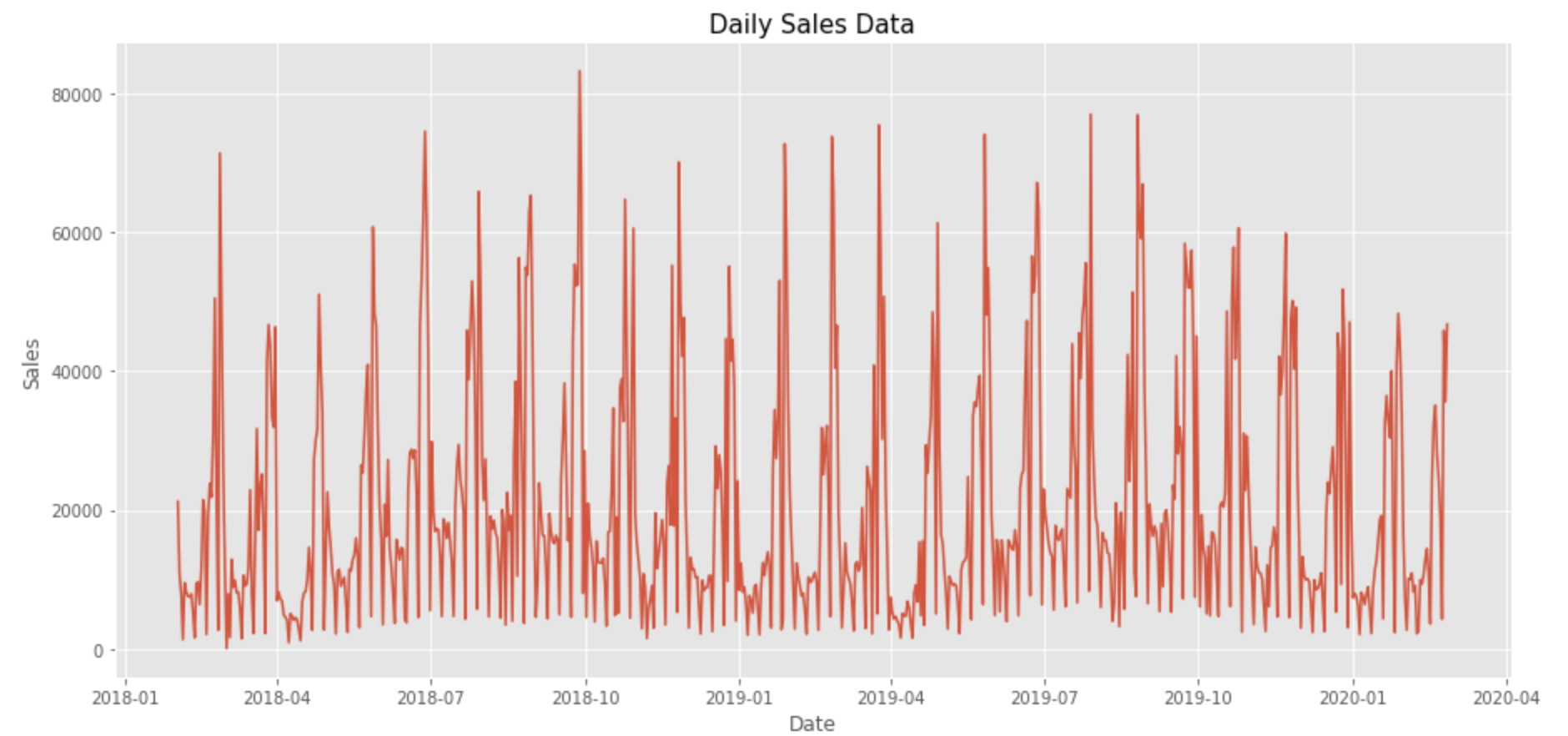
可視化して、年や月の周期性がありそうか確認します。
fig, ax = plt.subplots(figsize=(15,7))
a = sns.lineplot(x="Date", y="Sales", data=df)
a.set_title("Daily Sales Data",fontsize=15)
plt.show()
df['month'] = df.Date.apply(lambda x: x.month)
df['year'] = df.Date.apply(lambda x: x.year)
df['day'] = df.Date.apply(lambda x: x.day)
df['weekday'] = df.Date.apply(lambda x: x.dayofweek)

for i  in [2018,2019,2020]:
    example = df[df.year==i].copy()
    example.sort_values('Date',inplace=True)

    fig, (ax1, ax2, ax3) = plt.subplots(1, 3, figsize=(15, 4))
    example.groupby('day').mean()['Sales']\
        .plot(kind='line',
              title='average sale: day',
              lw=5,
              color='r',
              ax=ax1)

    example.groupby('month').mean()['Sales'] \
        .plot(kind='line',
              title='average sale: month',
              lw=5,
              color='g',

              ax=ax2)

    example.groupby('weekday').mean()['Sales'] \
        .plot(kind='line',
              lw=5,
              title='average sale: weekday',
              color='b',

              ax=ax3)

    fig.suptitle('Trends for year: {0}'.format(i),
                 size=20,
                 y=1.1)
    plt.tight_layout()
    plt.show()
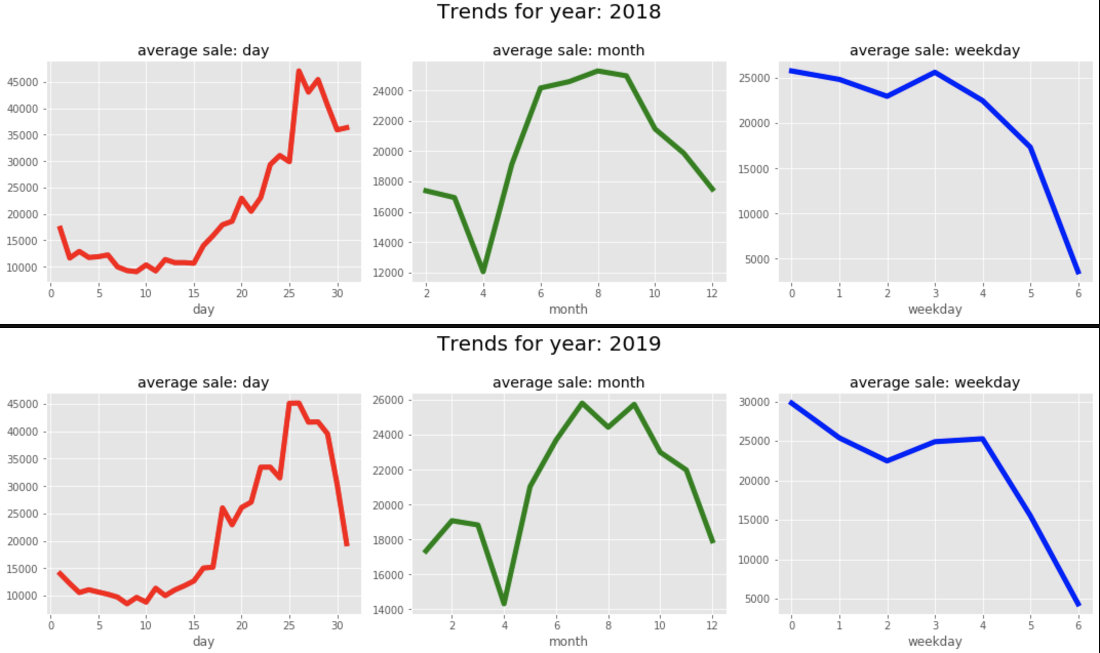
月の後半にかけて売上が上昇傾向にあり、1年を通じて夏に売上が隆起しています。また曜日ごとの周期性も確認できます。
Prophetで予測
Prophetでは、
-
ds:日付カラム -
y:予測対象カラム
を持つデータフレームを用意する必要があります。
また、学習を2018・2019年、テストを2020年に設定し、データを分割します。
df=df.rename(columns={'Date':'ds','Sales':'y'})
df = df[['ds','y']]
train_ord = df[df['ds'] < '2020-01-01']
test = df[df['ds'] >= '2020-01-01']
年・週ごとの季節性が見られたので、yearly_seasonality,weekly_seasonalityをTrueにして予測します。
m=Prophet(yearly_seasonality=True,weekly_seasonality=True)
m.fit(train_ord)
future = m.make_future_dataframe(periods=len(test))
forecast = m.predict(future)
forecast_plot = m.plot(forecast)
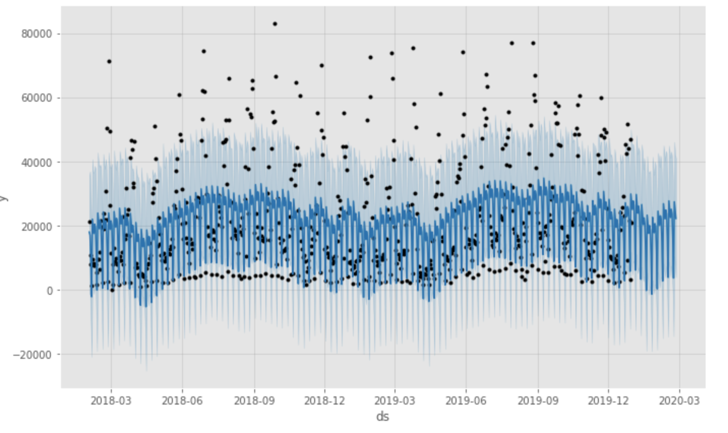
図の通り、デフォルトパラメータだとモデルはデータを正確にトレースできていません。
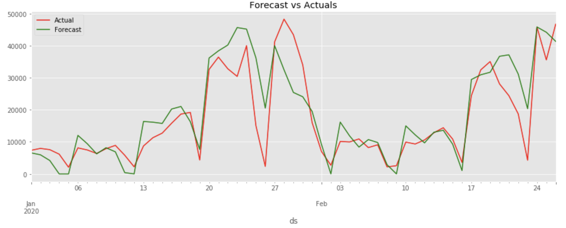
テスト期間(2020年)の予測値を、実測値と比較します。
test_forecast = forecast.tail(len(test))
test_forecast.loc[test_forecast['yhat'] < 0, 'yhat'] = 0

f, ax = plt.subplots(figsize=(14,5))
f.set_figheight(5)
f.set_figwidth(15)
test.plot(kind='line',x='ds', y='y', color='red', label='Actual', ax=ax)
test_forecast.plot(kind='line',x='ds',y='yhat', color='green',label='Forecast', ax=ax)
plt.title('Forecast vs Actuals')
plt.show()
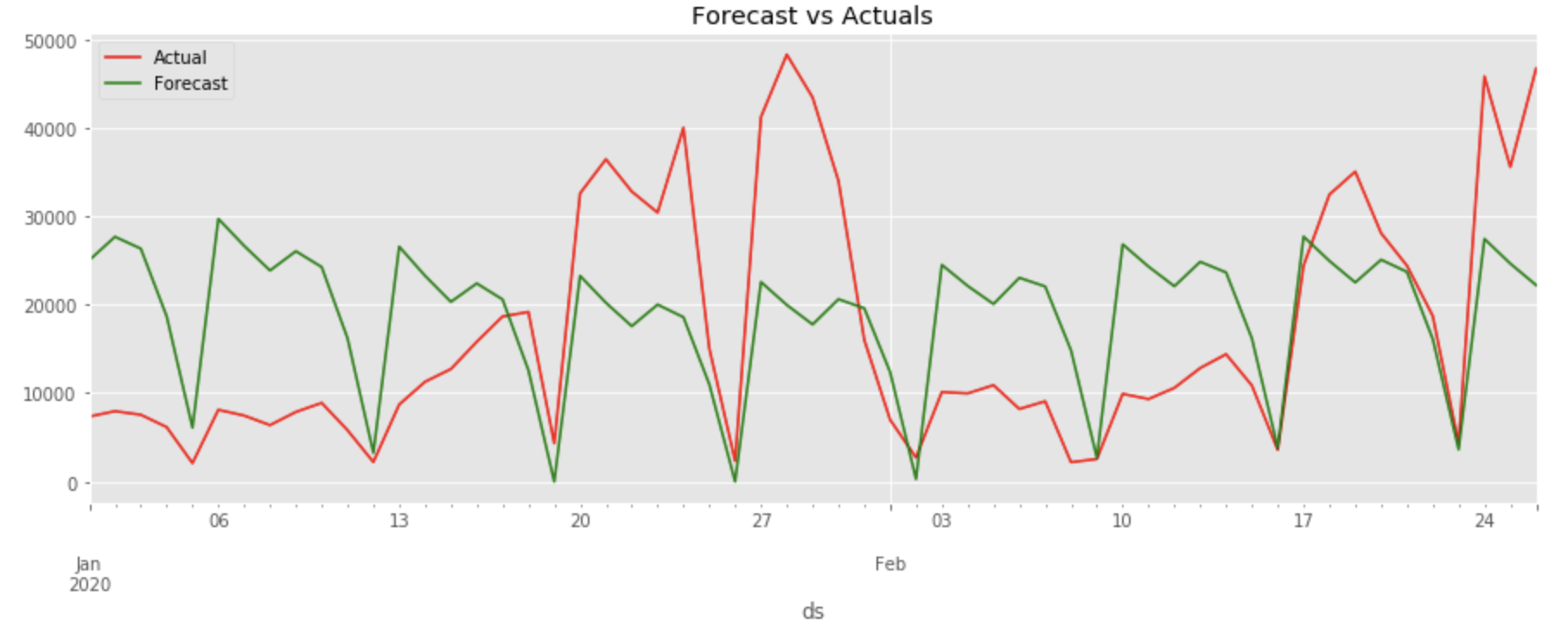
1月も2月も同じような周期で予測されてしまっています。モデルの学習が十分にされていないようです。
予測精度(MAPE)
np.mean(np.abs((test_forecast.yhat-test.y)/test.y))*100
104.9856312766537
Optunaによるパラメータチューニング
Prophetでは、季節性の事前分布や影響度・変化点検出に用いるデータの使用範囲・トレンドの影響など、チューニングできるパラメータが多くあります。特に、各パラメータが大きい影響力を持っていて、値を少し変えただけでも、予測値が大きく変化します。なので、Prophetでのパラメータチューニングは予測精度を高める上で重要なタスクになってきます。
Optunaとは
ハイパーパラメータの最適化を自動化するためのフレームワークです。
目的関数を定義し(def objective)、studyで最適化を実行します。今回はMAPEの最小化をしています。
今回チューニングするProphetの各パラメータ
-
changepoint_range
トレンドの変化点を検知するのに、どの範囲のデータを使用するかの割合
デフォルトは0.8で、最初の80%のデータを使用して傾向変化点を検出
公式によると[0.8、0.95]の範囲が妥当 -
n_changepoints
検出する変化点の候補の数を表すパラメータ
大きければ大きいほど多くの変化点が検出されやすくなる
デフォルトは25 -
changepoint_prior_scale
トレンドの柔軟性を制御するパラメータ
小さすぎるとトレンドが不十分であり、大きすぎるとトレンドが過剰適合してしまう
デフォルトは0.05で、公式によると[0.001、0.5]の範囲が妥当 -
seasonality_prior_scale
季節性の柔軟性を制御するパラメータ
デフォルトは10で、公式によると[0.01、10]の範囲が妥当 -
add_seasonality(period,fourier_order)
規定の年・週・日次の周期性だけでなく、任意の周期のモデルをユーザー自身で設定することが可能。
各周期性ごとに、周期性の単位(period)、季節成分の基礎となるフーリエ級数(fourier_order)、季節性の影響度(prior_scale)を設定。
各季節性のフーリエ級数と影響度を調整できるよう、規定の季節性を全てFalseにした上で、週・月・年・四半期の周期変動を追加してます。
※祝日・イベントに関するパラメータは今回扱いませんでした。
パラメータの探索範囲をそれぞれ指定して、Optunaを実装します。
def objective_variable(train,valid):

    cap = int(np.percentile(train.y,95))
    floor = int(np.percentile(train.y,5))


    def objective(trial):
            params = {
                    'changepoint_range' : trial.suggest_discrete_uniform('changepoint_range',0.8,0.95,0.001),
                    'n_changepoints' : trial.suggest_int('n_changepoints',20,35),
                    'changepoint_prior_scale' : trial.suggest_discrete_uniform('changepoint_prior_scale',0.001,0.5,0.001),
                    'seasonality_prior_scale' : trial.suggest_discrete_uniform('seasonality_prior_scale',1,25,0.5),
                    'yearly_fourier' : trial.suggest_int('yearly_fourier',5,15),
                    'monthly_fourier' : trial.suggest_int('monthly_fourier',3,12),
                    'weekly_fourier' : trial.suggest_int('weekly_fourier',3,7),
                    'quaterly_fourier' : trial.suggest_int('quaterly_fourier',3,10),
                    'yearly_prior' : trial.suggest_discrete_uniform('yearly_prior',1,25,0.5),
                    'monthly_prior' : trial.suggest_discrete_uniform('monthly_prior',1,25,0.5),
                    'weekly_prior' : trial.suggest_discrete_uniform('weekly_prior',1,25,0.5),
                    'quaterly_prior' : trial.suggest_discrete_uniform('quaterly_prior',1,25,0.5)
                     }
            # fit_model
            m=Prophet(
                    changepoint_range = params['changepoint_prior_scale'],
                    n_changepoints=params['n_changepoints'],
                    changepoint_prior_scale=params['changepoint_prior_scale'],
                    seasonality_prior_scale = params['seasonality_prior_scale'],
                    yearly_seasonality=False,
                    weekly_seasonality=False,
                    daily_seasonality=False,
                    growth='logistic',
                    seasonality_mode='additive')
            m.add_seasonality(name='yearly', period=365.25, fourier_order=params['yearly_fourier'],prior_scale=params['yearly_prior'])
            m.add_seasonality(name='monthly', period=30.5, fourier_order=params['monthly_fourier'],prior_scale=params['monthly_prior'])
            m.add_seasonality(name='weekly', period=7, fourier_order=params['weekly_fourier'],prior_scale=params['weekly_prior'])
            m.add_seasonality(name='quaterly', period=365.25/4, fourier_order=params['quaterly_fourier'],prior_scale=params['quaterly_prior'])

            train['cap']=cap
            train['floor']=floor

            m.fit(train)
            future = m.make_future_dataframe(periods=len(valid))

            future['cap']=cap
            future['floor']=floor

            forecast = m.predict(future)
            valid_forecast = forecast.tail(len(valid))

            val_mape = np.mean(np.abs((valid_forecast.yhat-valid.y)/valid.y))*100
            return val_mape

    return objective

def optuna_parameter(train,valid):
    study = optuna.create_study(sampler=optuna.samplers.RandomSampler(seed=42))
    study.optimize(objective_variable(train,valid), timeout=1000)
    optuna_best_params = study.best_params

    return study
検証データは、2019年12月の1ヶ月に設定しています。
train = df[df['ds'] < '2019-12-01']
valid = df[(df['ds'] >= '2019-12-01')&(df['ds'] < '2020-01-01')]
study = optuna_parameter(train,valid)
ベストパラメータが決まったら、再度予測します。
cap = int(np.percentile(train_ord.y,95))
floor = int(np.percentile(train_ord.y,5))

# fit_model
m=Prophet(
        changepoint_range = study.best_params['changepoint_prior_scale'],
        n_changepoints=study.best_params['n_changepoints'],
        seasonality_prior_scale = study.best_params['seasonality_prior_scale'],
        changepoint_prior_scale=study.best_params['changepoint_prior_scale'],
        yearly_seasonality=False,
        weekly_seasonality=False,
        daily_seasonality=False,
        growth='logistic',
        seasonality_mode='additive')
m.add_seasonality(name='yearly', period=365.25, fourier_order=study.best_params['yearly_fourier'],prior_scale=study.best_params['yearly_prior'])
m.add_seasonality(name='monthly', period=30.5, fourier_order=study.best_params['monthly_fourier'],prior_scale=study.best_params['monthly_prior'])
m.add_seasonality(name='weekly', period=7, fourier_order=study.best_params['weekly_fourier'],prior_scale=study.best_params['weekly_prior'])
m.add_seasonality(name='quaterly', period=365.25/4, fourier_order=study.best_params['quaterly_fourier'],prior_scale=study.best_params['quaterly_prior'])

train_ord['cap']=cap
train_ord['floor']=floor

m.fit(train_ord)
future = m.make_future_dataframe(periods=len(test))

future['cap']=cap
future['floor']=floor

forecast = m.predict(future)
forecast_plot = m.plot(forecast)
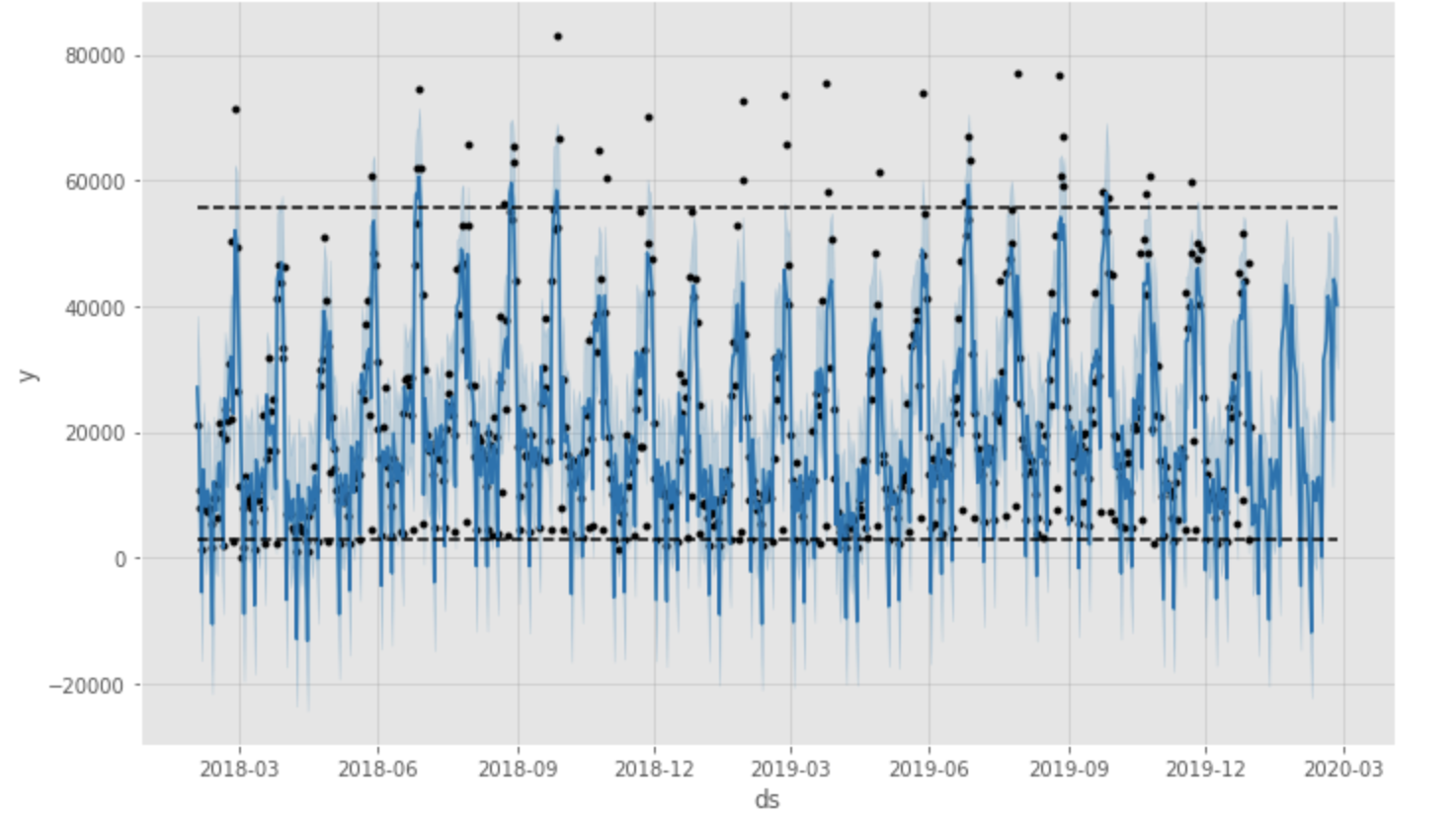
パラメータチューニング後の予測値と実測値との比較
予測精度(MAPE)
np.mean(np.abs((test_forecast.yhat-test.y)/test.y))*100
55.955005036694935
デフォルトの場合と比較して、約50%改善されています。それでも56%の誤差なので、予測精度が高いとは言えませんが。。
最後に
今回は、Optunaを用いてパラメータチューニングを行い、Prophetを実装しました。
Prophetはデフォルトパラメータのままでも簡単に実装できるのが特徴かと思いますが、パラメータチューニングを行うことで、さらにモデルの改善が期待できるかと思います。
最後まで読んでいただきありがとうございました。
引き続きアドベントカレンダーをお楽しみください。