初めまして。新入社員の石川です。
大学と大学院では半教師あり学習を専門にしてきました。今回はそのこれまでの技術と今後についてご紹介します。
半教師あり学習(Semi-Supervised Learning)とは
__半教師あり学習__は機械学習の手法の一つで、教師あり学習で必要となるデータ形成においてコスト削減を目指します。
まず、機械学習は大きく
- 教師あり学習
- 教師なし学習
- 強化学習
の3つが挙げられます。ここでは、__教師あり学習__と__教師なし学習__について簡単に説明した後に半教師あり学習について説明していきます。(強化学習は半教師あり学習とあまり関連がないため、別記事を参考にして下さい)
教師あり学習
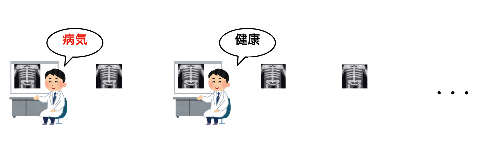
教師あり学習は、学習に必要となる教師データ(および評価データ)について全てのインスタンスに__アノテーション__と呼ばれるラベル付けの作業が必要です。
例えば、病院に来た患者のレントゲン写真をインプットしたときに、その患者が病気かどうかを分類する分類器を作る場合を考えます。教師あり学習ではこの分類器を作るために、学習データとして何かしらの方法で収集されたレントゲン写真を使用することになります。ただし、レントゲン写真だけをインプットするだけでは学習することはできません。これらのレントゲン写真1枚1枚に対して、それぞれが実際に病気の人のものであるかもしくはそうでないかという”ラベル”が必要だからです。このラベルを付加する作業をアノテーションと言います。
学習データの量が膨大でアノテーションが必要となる場合、教師あり学習はデータ形成の際に大きなコストが発生します。特に近年注目を集めているCNNを用いた画像分類などは、その分類性能の柔軟さのせいで大量の学習データの形成が必要となる場合があります。

教師なし学習
教師なし学習は教師あり学習とは対照的に、学習データ全てににラベルが付いていない状態で学習する手法です。クラスタリングともいいます。
例えば、映画のレコメンドに用いることができます。映画を見に行った人のこれまでの鑑賞履歴を大量のユーザに関して収集し、それを学習データとします。それらのデータから映画を見る人について「このような映画を見る人はこの映画を見る傾向がある」といったパターンを見つけ出し、それを用いてレコメンドの対象者におすすめの映画を提示することができます。
この手法はアノテーションを必要としないため、データ形成について教師あり学習よりもコスト面で有利となり得るけれども、全てのケースに用いることができるとは限らず、問題に適した手法を用いることが必要になります。
半教師あり学習
半教師あり学習は、文字通り教師あり学習と教師なし学習の間をとったような手法となっています。
具体的には半教師あり学習は大きく2種類挙げられて、
- 半教師あり分類学習
- 半教師ありクラスタリング
というものがあります。
半教師あり分類学習は、教師あり学習を拡張したもので学習データに必要となるラベルが一部にのみ付加されたもので学習をし、アノテーションにかかるコスト削減を目指します。対して半教師ありクラスタリングは、一部のデータ間にそれらが同じクラスタに属するかどうかの情報が付加されたもので学習をし、精度向上を目指します。
本稿では前者について扱います。また以後半教師あり学習と記すときは半教師あり分類学習を意味します。
前述したように、実社会において大量のデータにアノテーションが必要となる学習方法は実用的とはあまり言えません。しかしこのようなラベルの付いているデータを大量に収集するのが大変な一方で、ラベルの付いていないデータは比較的容易に手に入れることができます。そこで少数のラベル有りデータと多数のラベル無しデータによって構成された学習データを用いた学習方法である半教師あり学習が、学習データの収集の点で有利となりそうといえます。この半教師あり学習を利用することで、アノテーションにかかるコストを削減することができ、より実用性に優れた学習を実現することができると考えられます。
具体的な手法の例
半教師あり学習の手法を実現する方法として、下記のような手法が存在します。
- 自己訓練 (Self-Training)[1]
- 半教師あり混合ガウスモデル (semi-supervised Gaussian mixture models)[2]
- 共訓練 (Co-Training)[3]
- グラフベース半教師あり学習 (Graph-based Semi-Supervised Learning)[4]
- S3VM(Semi-Supervised Support Vector Machine)[5]
- PNU Learning[6]
PNU Learningを除いてはそれぞれ__モデル仮定__と呼ばれる仮定が必要です。モデル仮定とはラベル無しデータを学習に利用するためのデータに対する仮定であり、生成される分類器に対して大きな影響を与えて、真の仮定と大きく異なる仮定を採用した場合理想とは大きく異なる学習をすることが考えられます。対してPNU Learningはこのようなモデル仮定を必要としない半教師あり学習の手法として注目を集めています。
最近の半教師あり学習 "PNU Learning" の構成
ここでは私が個人的にすごいと思った手法のPNU Learningの構成について説明して、そのあとに実装例を紹介します。
- PNU Learningの予測損失
R_\mathrm{PNU}^\eta(g) := \left\{
\begin{array}{ll}
(1 - \eta) R_\mathrm{PN}(g) + \eta R_\mathrm{PU}(g) & \mathrm{if} \quad \eta \ge 0 \\
(1 + \eta) R_\mathrm{PN}(g) - \eta R_\mathrm{NU}(g) & \mathrm{otherwise}
\end{array}
\right.
上式に含まれる$R_\mathrm{PU}$、$R_\mathrm{NU}$、$R_\mathrm{PN}$はそれぞれPU Learning、NU Learning、PN Learningの予測損失に対応します。PU Learningは正のラベルを持つデータとラベルなしデータによる学習、NU Learningは負のラベルを持つデータとラベルなしデータによる学習、PN Learningは正のラベルを持つデータと負のラベルを持つデータによる学習で、これらを組み合わせて構成されています。この組み合わせの割合をハイパーパラメータ$\eta$によって調整できます。また、$g$はモデルになります。
- PN Learningの予測損失
R_\mathrm{PN}(g) := p(y=+1) R_\mathrm{P}^+(g) + p(y=-1) R_\mathrm{N}^-(g)
$p(y=+1)$、$p(y=-1)$ はそれぞれドメイン全体における正のラベルを持つ割合、負のラベルを持つ割合。ここで、
R_\mathrm{P}^+(g) := \mathbb{E}_\mathrm{P}\bigl[\ell\bigl(g({x}), +1\bigr)\bigr] \\
R_\mathrm{N}^-(g) := \mathbb{E}_\mathrm{N}\bigl[\ell\bigl(g({x}), -1\bigr)\bigr]
で、$ \ell\bigl(g({x}), +1\bigr) $は$ {x} $のラベルが正($+1$)のときの損失、 $\ell\bigl(g({x}), -1\bigr)$ は ${x}$ のラベルが負($-1$)のときの損失。
\mathbb{E}_\mathrm{P} と \mathbb{E}_\mathrm{N}
はそれぞれ正のラベルを持つデータの集合、負のラベルを持つデータの集合に対する期待値です。つまり、 $R_\mathrm{P}^+(g)$ と $R_\mathrm{N}^-(g)$ はそれぞれ正のラベルを持つデータに対する予測損失、負のラベルを持つデータに対する予測損失としてみることができます。
- PU Learningの予測損失
R_\mathrm{PU}(g) := p(y=+1) R_\mathrm{P}^+(g) + R_\mathrm{U}^-(g) - p(y=+1) R_\mathrm{P}^-(g)
これはPN Learningの予測損失を基にして確率の周辺化などを用いて導き出され、この予測損失は正のラベルを持つデータとラベルなしデータのみで算出できます。
ここで、
R_\mathrm{P}^-(g) := \mathbb{E}_\mathrm{P}\bigl[\ell\bigl(g({x}), -1\bigr)\bigr] \\
R_\mathrm{U}^-(g) := \mathbb{E}_\mathrm{U}\bigl[\ell\bigl(g({x}), -1\bigr)\bigr]
であり、$\mathbb{E}_\mathrm{U}$はラベルなしデータの集合に対する期待値です。
- NU Learningの予測損失
R_\mathrm{NU}(g) := p(y=-1) R_\mathrm{N}^-(g) + R_\mathrm{U}^+(g) - p(y=-1) R_\mathrm{N}^+(g)
これはPU Learningの予測損失と同様に導き出され、この予測損失は負のラベルを持つデータとラベルなしデータのみで算出できます。
ここで、
R_\mathrm{N}^+(g) := \mathbb{E}_\mathrm{N}\bigl[\ell\bigl(g({x}), +1\bigr)\bigr]\\
R_\mathrm{U}^+(g) := \mathbb{E}_\mathrm{U}\bigl[\ell\bigl(g({x}), +1\bigr)\bigr]
[6]の論文ではPNU Learningは実験的に多くのベンチマークのデータセットで、既存の半教師あり学習の手法に勝る正答率を記録していて、さらに汎化誤差の理論解析もされています。
PNU Learningの実装例
PNU LearningのPythonを用いた実装例は下の通りです。
分類に用いたデータセットはCIFAR-10で、今回はこの10クラス分類問題から2クラスを抽出し2クラス分類問題としました。モデルは畳み込み層を含む多層パーセプトロンです(コードを参照)。
- 必要ライブラリ
import time
import numpy as np
import tensorflow as tf
from keras import datasets      #データセットのダウンロードにのみ利用
- データの準備
(x_train, y_train), (x_test, y_test) = datasets.cifar10.load_data()
x_train = np.array(x_train).astype(np.float32) / 255.
y_train = y_train.reshape(-1)
x_train = x_train[y_train<=1]
y_train = y_train[y_train<=1]
y_train = [-1 if y==0 else 1 for y in y_train]
y_train = np.array(y_train).astype(np.int32)
x_test = np.array(x_test).astype(np.float32) / 255.
y_test = y_test.reshape(-1)
x_test = x_test[y_test<=1]
y_test = y_test[y_test<=1]
y_test = [-1 if y==0 else 1 for y in y_test]
y_test = np.array(y_test).astype(np.int32)

n_train = len(y_train)                  # number of train data
negative, positive = np.unique(y_train)
n_p = (y_train == positive).sum()       # number of positive
prior = float(n_p) / float(n_train)     # prior

input_shape = x_train.shape[1:]


# ラベルなしデータ生成

n_labeled = 100        # number of labeled data
n_unlabeled = 10000   # number of unlabeled data

n_p_labeled = int(prior * n_labeled)
n_n_labeled = n_labeled - n_p_labeled

# shuffle
perm = np.random.permutation(n_train)
x_train = x_train[perm]
y_train = y_train[perm]

# positive data as positive labeled data
x_p_labeled = x_train[y_train == positive][:n_p_labeled]

# negative data as positive labeled data
x_n_labeled = x_train[y_train == negative][:n_n_labeled]

# unlabeled data
if n_labeled + n_unlabeled == n_train:
    x_p_unlabeled = x_train[y_train == positive][n_p_labeled:]
    x_n_unlabeled = x_train[y_train == negative][n_n_labeled:]
elif n_unlabeled == n_train:
    x_p_unlabeled = x_train[y_train == positive]
    x_n_unlabeled = x_train[y_train == negative]
else:
    raise ValueError('Unsupported parameters n_labeled or n_unlabeled')

x_train = np.concatenate((x_p_labeled, x_n_labeled, x_p_unlabeled, x_n_unlabeled), axis=0)
y_train = np.concatenate((np.ones(n_p_labeled), -np.ones(n_n_labeled), np.zeros(n_unlabeled)), axis=0)

# shuffle
perm = np.random.permutation(len(y_train))
x_train = x_train[perm]
y_train = y_train[perm]
- モデル
def weight(shape=[]):
    return tf.Variable(tf.truncated_normal(shape, stddev = 0.01))

def conv_layer(X, W, out_channel, stride=1):
    conv = tf.nn.conv2d(X, W, [1, stride, stride, 1], padding='SAME')
    biases = weight([out_channel])
    return tf.nn.bias_add(conv, biases)

def cnn_model(X, input_shape, activation_name):

    if len(input_shape) != 3:
        raise ValueError('Unsuported data shape' + input_shape)

    if activation_name == 'relu':
        activation_function = tf.nn.relu
    elif activation_name == 'softsign':
        activation_function = tf.nn.softsign
    else:
        raise ValueError('Unsuported activation name')

    W1 = weight([3, 3, input_shape[-1], 96])
    W2 = weight([3, 3, 96, 192])
    W3 = weight([3, 3, 192, 192])
    W4 = weight([1, 1, 192, 10])
    W5 = weight([input_shape[0] // 2 * input_shape[1] // 2 * 10, 512])
    W6 = weight([512, 128])
    W7 = weight([128, 1])

    h = conv_layer(X, W1, 96, 1)
    h = tf.layers.BatchNormalization()(h,training=True)
    h = activation_function(h)
    h = conv_layer(h, W2, 192, 1)
    h = tf.layers.BatchNormalization()(h,training=True)
    h = activation_function(h)
    h = conv_layer(h, W3, 192, 2)
    h = tf.layers.BatchNormalization()(h,training=True)
    h = activation_function(h)
    h = conv_layer(h, W4, 10, 1)
    h = tf.layers.BatchNormalization()(h,training=True)
    h = activation_function(h)
    h = tf.reshape(h, [-1, input_shape[0] // 2 * input_shape[1] // 2 * 10])
    h = tf.matmul(h, W5)
    h = tf.layers.BatchNormalization()(h,training=True)
    h = activation_function(h)
    h = tf.matmul(h, W6)
    h = tf.layers.BatchNormalization()(h,training=True)
    h = activation_function(h)
    h = tf.matmul(h, W7)

    return h
- PNU Learningのクラス
class PNUlearn(object):

    def __init__(
        self, loss_name, minimizer_name, alpha,
        activation_name, input_shape, prior, eta=0
    ):

        self.loss_name = loss_name
        self.minimizer_name = minimizer_name
        self.alpha = alpha
        self.activation_name = activation_name
        self.input_shape = input_shape
        self.prior = prior
        self.eta = eta

    def t_P_index(self, t):
        return tf.maximum(t, tf.zeros_like(t))

    def t_N_index(self, t):
        return tf.maximum(-t, tf.zeros_like(t))

    def t_U_index(self, t):
        return tf.ones_like(t) - tf.abs(t)

    def R(self, index, y):
        n = tf.maximum(tf.reduce_sum(index), 1)
        return tf.divide(tf.reduce_sum(index * self.loss_func(-y)), n)

    def R_P_plus(self, t, y):
        return self.R(self.t_P_index(t), y)

    def R_P_minus(self, t, y):
        return self.R(self.t_P_index(t), -y)

    def R_N_plus(self, t, y):
        return self.R(self.t_N_index(t), y)

    def R_N_minus(self, t, y):
        return self.R(self.t_N_index(t), -y)

    def R_U_plus(self, t, y):
        return self.R(self.t_U_index(t), y)

    def R_U_minus(self, t, y):
        return self.R(self.t_U_index(t), -y)

    def R_PN(self, t, y):
        t = tf.reshape(t, [-1])
        y = tf.reshape(y, [-1])
        return self.prior * self.R_P_plus(t, y) + (1 - self.prior) * self.R_N_minus(t, y)

    def accuracy(self, t, y):
        t = tf.reshape(t, [-1])
        y = tf.reshape(y, [-1])
        return tf.reduce_mean(tf.maximum(tf.sign(y) * t, tf.zeros_like(t)))

    def R_PU(self, t, y):
        return self.prior * (self.R_P_plus(t, y) - self.R_P_minus(t, y)) + self.R_U_minus(t, y)

    def R_NU(self, t, y):
        return (1 - self.prior) * (self.R_N_minus(t, y) - self.R_N_plus(t, y)) + self.R_U_plus(t, y)

    def R_PNU(self):
        def PNPU(t, y):
            t = tf.reshape(t, [-1])
            y = tf.reshape(y, [-1])
            return (1 - self.eta) * self.R_PN(t, y) + self.eta * self.R_PU(t, y)
        def PNNU(t, y):
            t = tf.reshape(t, [-1])
            y = tf.reshape(y, [-1])
            return (1 + self.eta) * self.R_PN(t, y) - self.eta * self.R_NU(t, y)
        if self.eta >= 0:
            return PNPU
        else:
            return PNNU

    def fit(self, x_train, y_train, x_test, y_test, n_epoch, batch_size, verbose=True):

        start_fit = time.time()

        with tf.Session() as sess:

            x = tf.placeholder(tf.float32, [None, *self.input_shape])
            t = tf.placeholder(tf.float32, [None])

            if self.loss_name == 'sigmoid':
                self.loss_func = tf.nn.sigmoid
            else:
                raise ValueError('loss name ' + self.loss_name + ' is unknown.')

            out = cnn_model(x, self.input_shape, self.activation_name)
            train_loss_f = self.R_PNU()(t, out)
            test_loss_f = self.R_PN(t, out)
            test_acc_f = self.accuracy(t, out)

            if self.minimizer_name == 'adam':
                minimizer = tf.train.AdamOptimizer(learning_rate=self.alpha).minimize
            else:
                raise ValueError('minimizer name ' + self.minimizer_name + ' is unknown.')

            if self.eta == 0:
                updater = minimizer(self.R_PN(t, out))
            else:
                updater = minimizer(self.R_PNU()(t, out))

            n_train = x_train.shape[0]
            n_test = x_test.shape[0]
            history = np.empty((0,6))

            sess.run(tf.global_variables_initializer())

            train_time_sum = 0

            for epoch in range(1, n_epoch + 1):

                start_epoch = time.time()
                perm = np.random.permutation(n_train)

                for idx in range(0, n_train, batch_size):

                    if verbose:
                        bar_l = 30
                        progress = idx / n_train
                        bar = '>' * int(bar_l * progress) + ' ' * (bar_l - int(bar_l * progress))
                        print('\r{: >3} [{}] '.format(epoch, bar), end='')
                        print('{: >3}% {}/{}  '.format(int(100 * progress), idx, n_train), end='')
                        print('{:.2f}[sec]  '.format(time.time() - start_epoch), end='')
                    xi = x_train[perm[idx: idx + batch_size if idx + batch_size < n_train else n_train]]
                    ti = y_train[perm[idx: idx + batch_size if idx + batch_size < n_train else n_train]]

                    sess.run(updater, feed_dict = {x: xi, t: ti})

                train_time = time.time() - start_epoch
                train_time_sum += train_time
                if verbose:
                    print('\r{: >3} [{}] 100% {}/{}  '.format(epoch, '>' * bar_l, n_train, n_train), end='')
                    print('{:.2f}[sec]  '.format(train_time), end='')

                cal_size = 2000

                train_loss = 0
                for idx in range(0, n_train, cal_size):
                    xi = x_train[idx: idx + cal_size if idx + cal_size < n_train else n_train]
                    ti = y_train[idx: idx + cal_size if idx + cal_size < n_train else n_train]
                    train_loss += sess.run(train_loss_f, feed_dict = {x: xi, t: ti}) * xi.shape[0]
                train_loss = train_loss / n_train

                test_loss = 0
                test_acc = 0
                for idx in range(0, n_test, cal_size):
                    xi = x_test[idx: idx + cal_size if idx + cal_size < n_test else n_test]
                    ti = y_test[idx: idx + cal_size if idx + cal_size < n_test else n_test]
                    test_loss += sess.run(test_loss_f, feed_dict = {x: xi, t: ti}) * xi.shape[0]
                    test_acc += sess.run(test_acc_f, feed_dict = {x: xi, t: ti}) * xi.shape[0]
                test_loss = test_loss / n_test
                test_acc = test_acc / n_test

                epoch_time = time.time() - start_epoch

                history = np.vstack((
                        history,
                        np.array([epoch, train_loss, test_loss, test_acc, train_time, epoch_time])
                ))

                if verbose:
                    print('train_loss {: .3f}  '.format(train_loss), end='')
                    print('test_loss {: .3f}  '.format(test_loss), end='')
                    print('test_acc {: .3f}  '.format(test_acc), end='')
                    print('epoch_time {:.2f}[sec]'.format(epoch_time))

            train_time_ave = train_time_sum / n_epoch
            total_time = time.time() - start_fit
            if verbose:
                print('\nTotal time  {}h{: >2}m{: >2}s'.format(
                    int(total_time / 3600),
                    int(total_time / 60),
                    int(total_time % 60)
                ))
                print('Average train time  {:.3f}[sec]\n'.format(train_time_ave))

        return history
- 学習
learner = PNUlearn(
            loss_name='sigmoid',
            minimizer_name='adam',
            alpha=1e-05,
            activation_name='relu',
            input_shape=input_shape,
            prior=prior,
            eta=0.2
    )
history = learner.fit(
    x_train, y_train, x_test, y_test, n_epoch=10, batch_size=1000
)
学習結果
次のグラフは,上記のプログラムを実行したときのテストデータに対するAccuracyの変化です。

今回比較のために、ラベルなしデータ10,000件+ラベルありデータ100件による半教師あり学習と、ラベルありデータ100件のみによる教師あり学習をしました。グラフからは半教師あり学習が教師あり学習のAccuracyを上回る様子が見られて、ラベルなしデータが学習に良い効果をもたらしていることがわかります。
まとめ
半教師あり学習は、教師データ全てにラベル付けをする必要がないため最近注目を集めている分野で、特に教師データ全体に対して1%程度のデータにラベルが付いているもので学習することを目指している手法も多くあり、アノテーションにかかるコストを大幅に削減することができそうです。
また、例に挙げたような手法の具体例はそれぞれ問題に対して適している適していないがあり、ここに注意して学習手法の選択できればと思います。
半教師あり学習は、今後オンライン学習への組み込みや回帰問題への適用など様々な展開の余地があり、この分野の発展に期待できます。
参考文献
[1] Xiaojin Zhu. Semi-supervised learning literature survey. Computer Science, University of Wisconsin-Madison, Vol.2, No.3, p.4, 2006.
[2] Kamal Nigam, Andrew Kachites McCallum, Sebastian Thrun, and Tom Mitchell. Text classification from labeled and unlabeled documents using em. Machine learning, Vol.39, No.2-3, pp.103–134, 2000.
[3] Avrim Blum and Tom Mitchell. Combining labeled and unlabeled data with co-training. In Pro-ceedings of the eleventh annual conference on Computational learning theory, pp.92–100. ACM, 1998.
[4] Xiaojin Zhu, Zoubin Ghahramani, and John D Lafferty. Semi-supervised learning using gaussian fields and harmonic functions. In Proceedings of the 20th International conference on Machine learning (ICML-03), pp.912–919,2003.
[5] Kristin P Bennett and Ayhan Demiriz. Semi-supervised support vector machines. In Advances in Neural Information processing systems, pp.368–374, 1999.
[6] Tomoya Sakai, Marthinus Christoffel du Plessis, Gang Niu, and Masashi Sugiyama. Semi-supervised classification based on classification from positive and unlabeled data. In Proceedings of the 34th International Conference on Machine Learning, ICML 2017, Sydney, NSW, Australia, 6-11 August 2017, pp.2998–3006, 2017.
[7] 石川 周, 全 眞嬉, 徳山 豪, 制約付き最適化を用いた非負PNU半教師学習による過学習の抑制, The 81st National Convention of IPSJ