Pythonで標準偏差を理解してみる

標準偏差とは

https://ja.wikipedia.org/wiki/標準偏差
標準偏差（ひょうじゅんへんさ、（英: standard deviation, SD）とは、データや確率変数の、平均値からの散らばり具合（ばらつき）を表す指標の一つである。偏差ベクトルと、値が標準偏差のみであるベクトルは、ユークリッドノルムが等しくなる。
標準偏差を2乗したのが分散であり、従って、標準偏差は分散の非負の平方根である[1]。標準偏差が 0 であることは、データの値が全て等しいことと同値である。
母集団や確率変数の標準偏差を σ で、標本の標準偏差を s で表すことがある。
二乗平均平方根 (RMS) を用いると、標準偏差は偏差の二乗平均平方根に等しくなる。

なるほどわからん。
どうやら平均からどれだけデータがばらついているかを表す指標ということらしい。

平均は文系の私でもまあわかる。
標準偏差は次の式で求められるみたいだが…。

…まあこれは置いといてnumpyのstd()で求められるので試してみる。

import numpy

scores = [
  {
      "label": "【A.均等にばらついてるデータ】",
      "data": [
        20, 30, 40, 50, 60,
        60, 70, 80, 90, 100,
      ],
  },
  {
      "label": "【B.一部が平均以下のデータ】",
      "data": [
        0, 5, 10, 70, 80, 
        80, 82, 85, 93, 95,
      ],
  },
  {
      "label": "【C.一部が平均以上のデータ】",
      "data": [
        50, 52, 54, 60, 60,
        60, 61, 61, 70, 72,
      ],
  },
]

def print_mean_and_std(label, data):
  print(label)

  mean = numpy.average(data)
  print("平均：%s" % mean)

  std = numpy.std(data)
  print("標準偏差：%s" % std)

for score in scores:
  print_mean_and_std(score["label"], score["data"])

【A.均等にばらついてるデータ】
平均：60.0
標準偏差：24.49489742783178
【B.一部が平均以下のデータ】
平均：60.0
標準偏差：36.67151483099655
【C.一部が平均以上のデータ】
平均：60.0
標準偏差：6.6783231428256

で、この標準偏差で出てきた数値がなんなんだってばよ…。

調べると標準偏差が求まることで、平均±標準偏差の範囲にデータの分布が集中していることがわかるそう。

つまり上記の例のCならば60.0±6.6783231428256なので52.3～66.6の間に分布が集中していることになると。
うん、確かに。

正規分布

これをわかりやすくするために正規分布というグラフにしてみる。

#!pip install japanize-matplotlib

import matplotlib.pyplot as plt
import japanize_matplotlib
import numpy
from scipy.stats import norm

scores = [
  {
      "label": "【A.均等にばらついてるデータ】",
      "data": [
        20, 30, 40, 50, 60,
        60, 70, 80, 90, 100,
      ],
  },
  {
      "label": "【B.一部が平均以下のデータ】",
      "data": [
        0, 5, 10, 70, 80, 
        80, 82, 85, 93, 95,
      ],
  },
  {
      "label": "【C.一部が平均以上のデータ】",
      "data": [
        50, 52, 54, 60, 60,
        60, 61, 61, 70, 72,
      ],
  },
]

def plot_hist(label, data):
  mean = numpy.average(data)
  std = numpy.std(data)

  fig, ax = plt.subplots()
  ax.set_title(label)
  ax.set_xlabel("得点")
  ax.set_ylabel("割合")

  bins = numpy.arange(0, 101)
  plt.hist(data, bins, density=True)

  xn = numpy.linspace(min(bins), max(bins), 100)
  yn = norm.pdf(xn, loc=mean, scale=std)

  plt.plot(xn, yn)
  plt.show()

for score in scores:
  plot_hist(score["label"], score["data"])

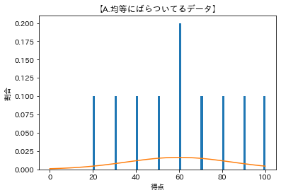
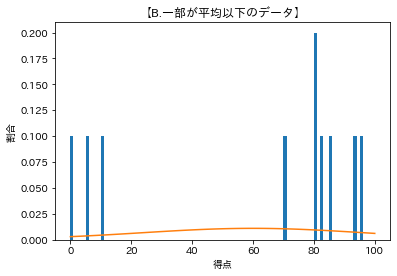
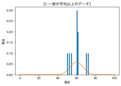
カーブのてっぺんが平均値の位置で、標準偏差が大きいほどばらついてるのでカーブの幅が広くなっている。

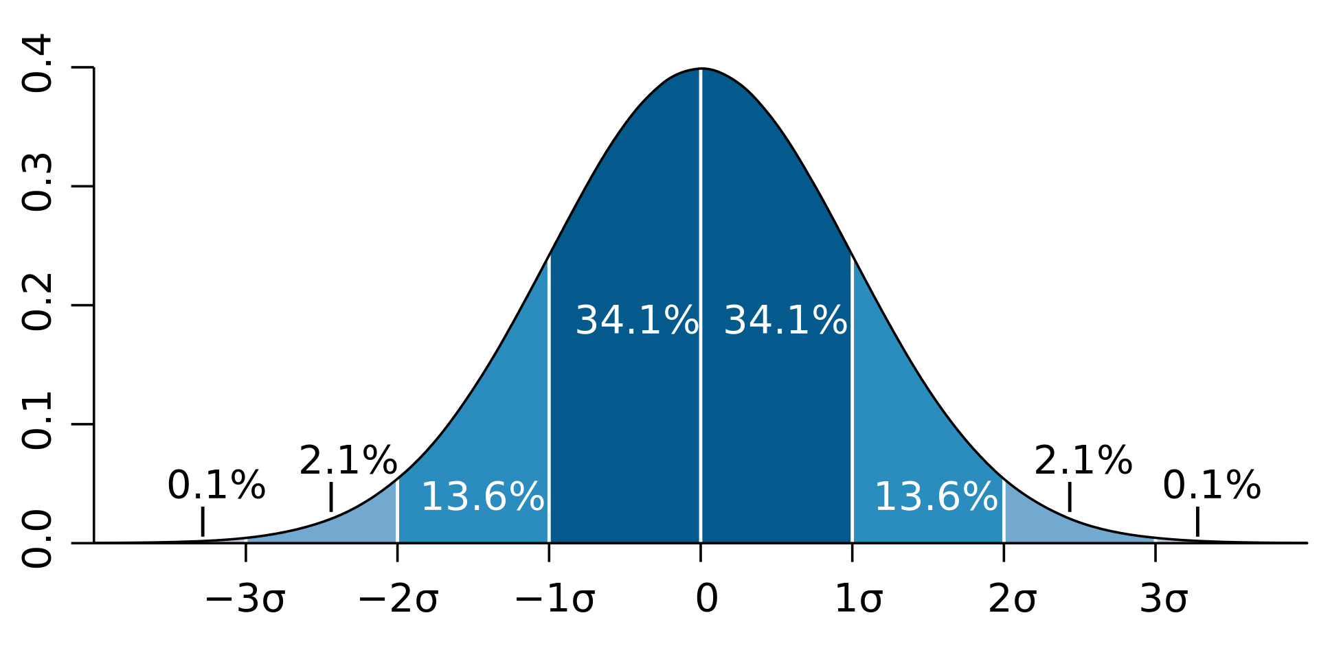
1σ、2σ、3σ

標準偏差×1したものを1σ。
×2したものを2σ、×3したものを3σと呼ぶそう。

で、それぞれの区間に分布が収まる確率が

• 1σ ＝ 約68%
• 2σ ＝ 約95%
• 3σ ＝ 約99.7%

となり、この法則は平均や標準偏差の値が何であれ成り立つそう。
68–95–99.7則とも呼ばれる。

まとめ

標準偏差を理解するために書いてみました。
数式だととっつきづらいけど、Notebookにコードを書きながら学んでみると何となく理解できるもんですね。

参考