1. はじめに
最近仕事で作ったグラフを紹介します.
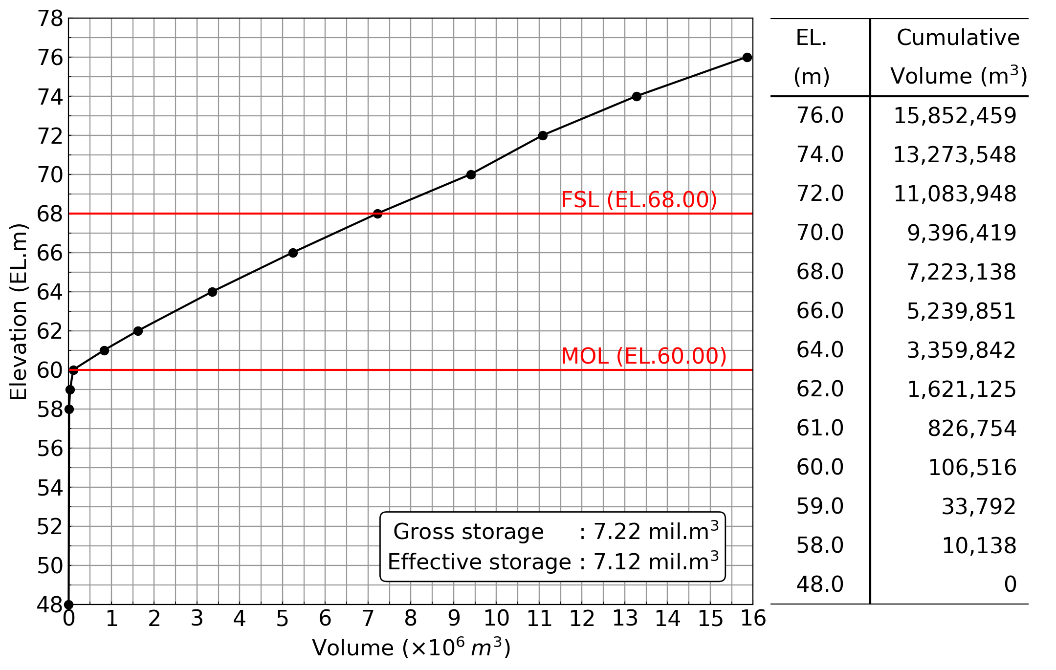
作品は以下の画像です.
このグラフの作図上のポイントは以下の3点です.
- グラフの右側に表形式でプロット点を記載している
- グリッドを補助目盛りにも入れている
- 右下に複数行の文字列をボックスの中に表示している
2. グラフ作成の解説
(1) モジュールのインポートする
- numpy と matplotlib pyplot はセットで読み込む
- グリッドを制御するため ticker を読み込む
- 線形補間を行うため scipy interpolate を読み込む
import numpy as np
import matplotlib.pyplot as plt
import matplotlib.ticker as tick
from scipy import interpolate
(2) 作図用データを作成
後ほど図に表示するための数値 s_gross と s_effec を計算しておく
_el=np.array([48,58,59,60,61,62,64,66,68,70,72,74,76])
_vv=np.array([0,10138,33792,106516,826754,1621125,3359842,5239851,7223138,9396419,11083948,13273548,15852459])
s_gross=_vv[8]/1e6
s_effec=(_vv[8]-_vv[3])/1e6
(3) 線形補間(おまけ)
データが飛び飛びなので,0.5mピッチで線形補間する
f=interpolate.interp1d(_el,_vv)
el=np.arange(48,76+0.5,0.5)
vv=f(el)
(4) 表を作成するためのデータをリストに保存
str1=[]
str2=[]
for i in range(0,len(_el)):
    str1=str1+['{0:6.1f}'.format(_el[i])]
    str2=str2+['{0:,}'.format(_vv[i])]
str1=str1+['(m)']
str2=str2+['Volume (m$^3$)']
str1=str1+['EL.']
str2=str2+['Cumulative']
(5) 他の計算で使うため,0.5mピッチで線形補間したデータをファイルに保存.
fnameW='inp_RHV.txt'
fw=open(fnameW,'w')
print('{0}'.format(1),file=fw)
for i in range(0,len(el)):
    print('{0:6.1f}{1:12.0f}'.format(el[i],vv[i]),file=fw)
fw.close()
(6) 作図領域の定義
フォントサイズ(fsz),画像の保存ファイル名(fnameF),画像サイズなどを指定.
ここで,グラフ部分を画像領域の左70%としてax1で,表部分を画像領域の右30%としてax2で定義する.
fsz=16
fnameF='fig_RHV.png'
fig=plt.figure(figsize=(10,6),facecolor='w')
plt.rcParams["font.size"] = fsz
plt.rcParams['font.family'] ='sans-serif'
ax1=fig.add_axes((0.0, 0.0, 0.7, 1.0))
ax2=fig.add_axes((0.7, 0.0, 0.3, 1.0))
(7) ax1の描画
a. グリッド描画
ここで,グリッドの描画は以下で行っている.
- 横軸主目盛り間隔をdv=1,縦軸主目盛り間隔をde=2とする.
- 横軸補助目盛り間隔をdv/2=0.5,縦軸補助目盛り間隔をde/2=1とする
- gridで主目盛り・補助目盛り双方を灰色の実線で描画する.
ax1.xaxis.set_major_locator(tick.MultipleLocator(dv))
ax1.yaxis.set_major_locator(tick.MultipleLocator(de))
ax1.xaxis.set_minor_locator(tick.MultipleLocator(dv/2))
ax1.yaxis.set_minor_locator(tick.MultipleLocator(de/2))
ax1.grid(which='both',color='#999999',linestyle='solid')
b. グラフ右下の枠内への文字列の表示
- 文字列s1およびs2を定義
- 文字列s1とs2を
\nで連結する(これで2行表示となる) - propsで文字列を書き込む枠の形式を定義
- textで文字列描画.この際transformを用いグラフ領域の相対座標(左下が[0,0],右上が[1,1])で文字列描画位置を指定する
s1='Gross storage     : {0:4.2f} mil.m$^3$'.format(s_gross)
s2='Effective storage : {0:4.2f} mil.m$^3$'.format(s_effec)
textstr=s1+'\n'+s2
props = dict(boxstyle='round', facecolor='#ffffff', alpha=1)
ax1.text(0.95, 0.05, textstr, transform=ax1.transAxes, fontsize=fsz,va='bottom',ha='right', bbox=props)
(8) ax2に表を描画する
まず描画範囲を指定し,axis('off')で座標軸を描画しないようにする.
xmin=0; xmax=5
ymin=0; ymax=len(str1)
ax2.axis('off')
ax2.set_xlim(xmin,xmax)
ax2.set_ylim(ymin,ymax)
リストに格納した文字列を描画後,以下により横線と縦線を描画.
複数の横線や縦線を引くにはhlines, vlines が便利.
seqy=np.array([ymax,ymax-2,ymin])
seqx=np.array([2])
plt.hlines(seqy, xmin+0.3, xmax-0.3, colors="k", linestyle="solid")
plt.vlines(seqx, ymin, ymax, colors="k", linestyle="solid")
3. プログラム全文.
# =======================================
# Reservoir Capacity Curve
# =======================================
import numpy as np
import matplotlib.pyplot as plt
import matplotlib.ticker as tick
from scipy import interpolate

# latest (28 August 2017)
_el=np.array([48,58,59,60,61,62,64,66,68,70,72,74,76])
_vv=np.array([0,10138,33792,106516,826754,1621125,3359842,5239851,7223138,9396419,11083948,13273548,15852459])
s_gross=_vv[8]/1e6
s_effec=(_vv[8]-_vv[3])/1e6

f=interpolate.interp1d(_el,_vv)
el=np.arange(48,76+0.5,0.5)
vv=f(el)

str1=[]
str2=[]
for i in range(0,len(_el)):
    str1=str1+['{0:6.1f}'.format(_el[i])]
    str2=str2+['{0:,}'.format(_vv[i])]
str1=str1+['(m)']
str2=str2+['Volume (m$^3$)']
str1=str1+['EL.']
str2=str2+['Cumulative']


fnameW='inp_RHV.txt'
fw=open(fnameW,'w')
print('{0}'.format(1),file=fw)
for i in range(0,len(el)):
    print('{0:6.1f}{1:12.0f}'.format(el[i],vv[i]),file=fw)
fw.close()


fsz=16
fnameF='fig_RHV.png'
fig=plt.figure(figsize=(10,6),facecolor='w')
plt.rcParams["font.size"] = fsz
plt.rcParams['font.family'] ='sans-serif'
ax1=fig.add_axes((0.0, 0.0, 0.7, 1.0))
ax2=fig.add_axes((0.7, 0.0, 0.3, 1.0))

vmin=0.0;vmax=16.0;dv=1.0
emin=48.0;emax=78.0;de=2.0
ax1.set_xlabel('Volume ($\\times 10^6\: m^3$)')
ax1.set_ylabel('Elevation (EL.m)')
ax1.set_xlim(vmin,vmax)
ax1.set_ylim(emin,emax)

ax1.xaxis.set_major_locator(tick.MultipleLocator(dv))
ax1.yaxis.set_major_locator(tick.MultipleLocator(de))
ax1.xaxis.set_minor_locator(tick.MultipleLocator(dv/2))
ax1.yaxis.set_minor_locator(tick.MultipleLocator(de/2))
ax1.grid(which='both',color='#999999',linestyle='solid')

ax1.plot(_vv/1e6,_el,'ko', clip_on=False)
ax1.plot(vv/1e6,el,'k',clip_on=False)
ax1.plot([vmin,vmax],[60,60],color='#ff0000')
ax1.plot([vmin,vmax],[68,68],color='#ff0000')
ax1.text(11.5,60.1,'MOL (EL.60.00)',color='#ff0000',ha='left',va='bottom',fontsize=fsz)
ax1.text(11.5,68.1,'FSL (EL.68.00)',color='#ff0000',ha='left',va='bottom',fontsize=fsz)
s1='Gross storage     : {0:4.2f} mil.m$^3$'.format(s_gross)
s2='Effective storage : {0:4.2f} mil.m$^3$'.format(s_effec)
textstr=s1+'\n'+s2
props = dict(boxstyle='round', facecolor='#ffffff', alpha=1)
ax1.text(0.95, 0.05, textstr, transform=ax1.transAxes, fontsize=fsz,va='bottom',ha='right', bbox=props)

xmin=0; xmax=5
ymin=0; ymax=len(str1)
ax2.axis('off')
ax2.set_xlim(xmin,xmax)
ax2.set_ylim(ymin,ymax)
for i in range(len(str2)):
    if len(str2)-2<=i:
        ax2.text(1.0,i+0.2,str1[i],ha='center',va='bottom',fontsize=fsz)
        ax2.text(3.5,i+0.2,str2[i],ha='center',va='bottom',fontsize=fsz)
    else:
        ax2.text(xmin+0.5,i+0.2,str1[i],ha='left',va='bottom',fontsize=fsz)
        ax2.text(xmax-0.5,i+0.2,str2[i],ha='right',va='bottom',fontsize=fsz)

seqy=np.array([ymax,ymax-2,ymin])
seqx=np.array([2])
plt.hlines(seqy, xmin+0.3, xmax-0.3, colors="k", linestyle="solid")
plt.vlines(seqx, ymin, ymax, colors="k", linestyle="solid")

plt.savefig(fnameF, dpi=200, bbox_inches="tight", pad_inches=0.1)
plt.show()
4. もう一つの方法(プログラム全文)
plt だけで書いてしまう.個人的にはこちらのほうが好きです.
# =======================================
# Reservoir Capacity Curve
# =======================================
import numpy as np
import matplotlib.pyplot as plt
import matplotlib.ticker as tick
from scipy import interpolate


def drawfig1(_el,_vv,el,vv,fsz):
    xmin=0.0;xmax=16.0;dx=1.0
    ymin=48.0;ymax=78.0;dy=2.0
    plt.xlabel('Volume ($\\times 10^6\: m^3$)')
    plt.ylabel('Elevation (EL.m)')
    plt.xlim(xmin,xmax)
    plt.ylim(ymin,ymax)
    plt.xticks(np.arange(xmin,xmax+dx,dx))
    plt.yticks(np.arange(ymin,ymax+dy,dy))
    plt.gca().xaxis.set_minor_locator(tick.MultipleLocator(dx/2))
    plt.gca().yaxis.set_minor_locator(tick.MultipleLocator(dy/2))
    plt.grid(which='both',color='#999999',linestyle='solid')
    plt.plot(_vv/1e6,_el,'ko', clip_on=False)
    plt.plot(vv/1e6,el,'k-',clip_on=False)
    plt.plot([xmin,xmax],[60,60],color='#ff0000')
    plt.plot([xmin,xmax],[68,68],color='#ff0000')
    plt.text(11.5,60.1,'MOL (EL.60.00)',color='#ff0000',ha='left',va='bottom',fontsize=fsz)
    plt.text(11.5,68.1,'FSL (EL.68.00)',color='#ff0000',ha='left',va='bottom',fontsize=fsz)
    s_gross=_vv[8]/1e6
    s_effec=(_vv[8]-_vv[3])/1e6
    s1='Gross storage     : {0:4.2f} mil.m$^3$'.format(s_gross)
    s2='Effective storage : {0:4.2f} mil.m$^3$'.format(s_effec)
    textstr=s1+'\n'+s2
    props = dict(boxstyle='round', facecolor='#ffffff', alpha=1)
    xs=xmin+0.95*(xmax-xmin); ys=ymin+0.05*(ymax-ymin)
    plt.text(xs,ys, textstr, fontsize=fsz,va='bottom',ha='right', bbox=props)


def drawfig2(str1,str2,fsz):
    xmin=0; xmax=5
    ymin=0; ymax=len(str1)
    plt.axis('off')
    plt.xlim(xmin,xmax)
    plt.ylim(ymin,ymax)
    for i in range(len(str2)):
        if len(str2)-2<=i:
            plt.text(1.0,i+0.2,str1[i],ha='center',va='bottom',fontsize=fsz)
            plt.text(3.5,i+0.2,str2[i],ha='center',va='bottom',fontsize=fsz)
        else:
            plt.text(xmin+0.5,i+0.2,str1[i],ha='left',va='bottom',fontsize=fsz)
            plt.text(xmax-0.5,i+0.2,str2[i],ha='right',va='bottom',fontsize=fsz)
    seqy=np.array([ymax,ymax-2,ymin])
    seqx=np.array([2])
    plt.hlines(seqy, xmin+0.3, xmax-0.3, colors="k", linestyle="solid")
    plt.vlines(seqx, ymin, ymax, colors="k", linestyle="solid")


def figcontrol(_el,_vv,el,vv,str1,str2):
    fsz=16
    fnameF='fig_RHV.png'
    fig=plt.figure(figsize=(10,6),facecolor='w')
    plt.rcParams["font.size"] = fsz
    plt.rcParams['font.family'] ='sans-serif'
    plt.axes((0.0, 0.0, 0.7, 1.0)); drawfig1(_el,_vv,el,vv,fsz)
    plt.axes((0.7, 0.0, 0.3, 1.0)); drawfig2(str1,str2,fsz)
    plt.savefig(fnameF, dpi=200, bbox_inches="tight", pad_inches=0.1)
    plt.show()


def main():
    # latest (28 August 2017)
    _el=np.array([48,58,59,60,61,62,64,66,68,70,72,74,76])
    _vv=np.array([0,10138,33792,106516,826754,1621125,3359842,5239851,7223138,9396419,11083948,13273548,15852459])
    # linear interpolation with elevation interval of 0.5m
    f=interpolate.interp1d(_el,_vv)
    el=np.arange(48,76+0.5,0.5)
    vv=f(el)
    # makeing list for table drawing
    str1=[]
    str2=[]
    for i in range(0,len(_el)):
        str1=str1+['{0:6.1f}'.format(_el[i])]
        str2=str2+['{0:,}'.format(_vv[i])]
    str1=str1+['(m)']
    str2=str2+['Volume (m$^3$)']
    str1=str1+['EL.']
    str2=str2+['Cumulative']
    # data saving for other programs
    fnameW='inp_RHV.txt'
    fw=open(fnameW,'w')
    print('{0}'.format(1),file=fw)
    for i in range(0,len(el)):
        print('{0:6.1f}{1:12.0f}'.format(el[i],vv[i]),file=fw)
    fw.close()
    # figure control
    figcontrol(_el,_vv,el,vv,str1,str2)


# ==============
# Execution
# ==============
if __name__ == '__main__': main()
以 上