はじめに
最近、日単位の雨量データや流量データなどを、月別で整理することがあるのだが、その時使っているプログラムを紹介する。一つはヒートマップ、もう一つは折れ線グラフである。
ヒートマップはseabornのヒートマップを用いている。公式サイトは以下の場所。
https://seaborn.pydata.org/generated/seaborn.heatmap.html
作例
作例は以下の通り。
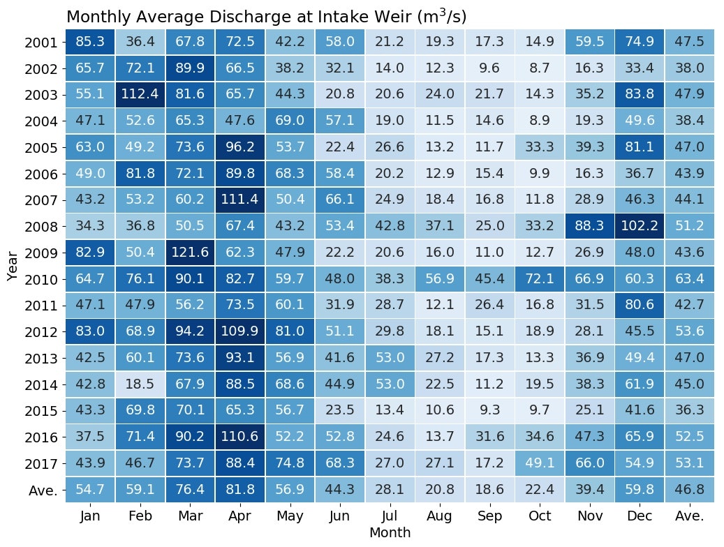
上段の図は、縦軸を年、横軸を月として、ある河川の各月の平均流量を表示したもの。最右列は各年の平均流量を、最下段は各月の平均流量を表示している。このような数値は、エクセルやワードの表として整理されていることが多いと思うが、報告書への貼り付けあるいはプレゼン用の表として用いるのならば、処理は計算機で行っているので、そのまま画像出力してしまったほうが楽である(と思う)。
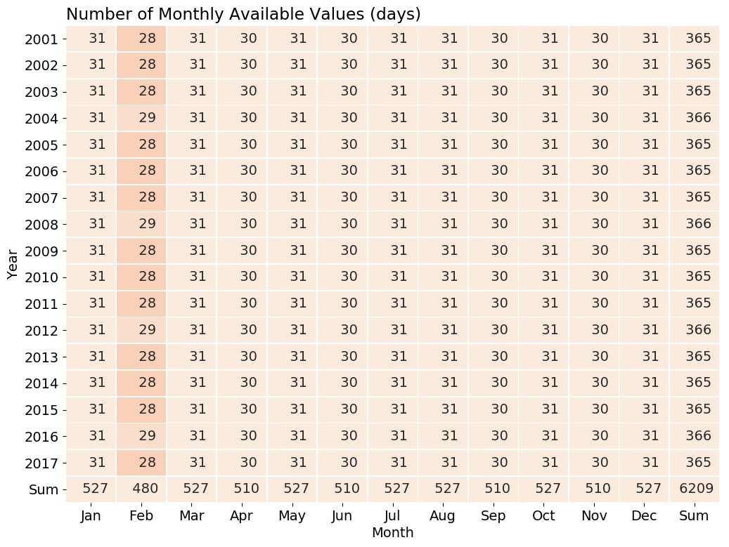
中段の図は、各月のデータの有効日数を表示したもの。この事例では2001年1月1日から2017年12月31日まで全ての日のデータが有効となっているが、欠測日(流量値がゼロ以下もしくはnan)があれば日付が少なく表示される。
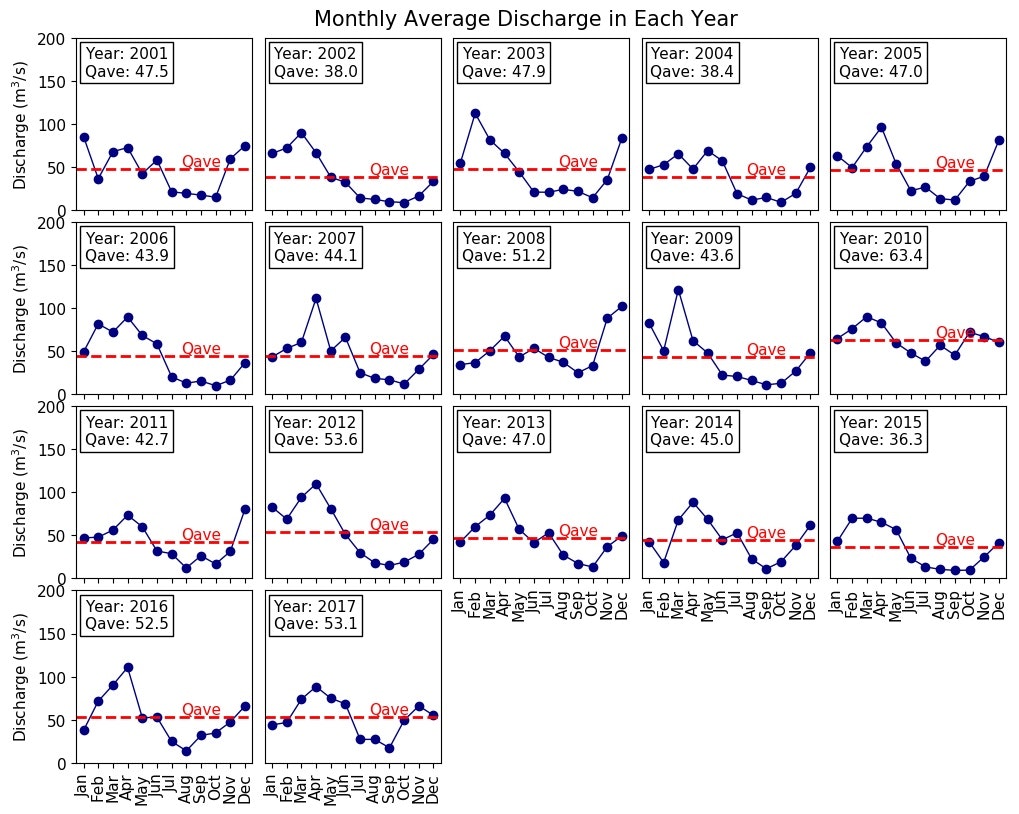
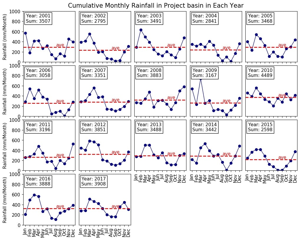
下段の図は、1年毎の月別平均流量の推移を折れ線グラフで表示し、それをsubplotで並べたもの。連続的な時系列図とするよりも、各年の特徴が見やすくなっている(と思う)。
流量データ表示プログラム
グローバル変数
分析したい年を文字列リストに格納。文字列を打ち込むのがめんどうなのでNumpy配列を作っておき、これを文字列に変換している。
関数:rdata
- csvとして保存されているデータファイルをpandasのデータフレームとして読み込む。
- ファイルには1列目には似付、2列目以降に各種データが日付順に格納されている。
- 読み込み時に1列目(日付列)を index_col=0 によりインデックスに指定。
- 読み込んだ時点では日付はただの文字列なので、pd.to_datetime で日付として認識させる。
- この事例では、データは2000年3月1日から始まっているが、年間を通してのデータがほしいので、インデックスを用いて2000年12月31日以前のデータは捨てる
- 戻り値は、実際に分析で用いる日付と流量だけのシリーズにしている。
関数:makedf
- データを各年・各月別に整理して「画面出力」に示すようなデータフレームを作成する。
- 月平均を出す際にはmeanは使わず、各月で有効なデータの合計と有効なデータを有する 日数を記憶させ、あとで合計を日数で除すことにより平均を求めている。
- 戻り値は、月別平均値を格納したデータフレームと、月別有効日数を格納したデータフレーム。
関数:fighmap1
月別平均流量を表示するヒートマップ。水なので色はブルー系。
関数:fighmap2
月別有効日数(有効なデータが入っている日数)を表示するヒートマップ。色はデフォルト。
関数:figts
- 1年1グラフで月別流量をしめす時系列図をsubplotで並べたもの。
- この事例では17年分、17枚のグラフを並べるため、配置を4行5列(グラフ20枚分)としている。
- 座標軸を全グラフに入れるのはうるさいので、縦軸は左端グラフのみ、横軸は一番下になるグラフのみに入れている。
関数:main
制御部。
プログラム全文
# Outline of flow data
import numpy as np
import pandas as pd
import datetime
import matplotlib.pyplot as plt
import seaborn as sns


# global
_ylist=np.arange(2001,2018,1)
ylist=[]
for y in _ylist:
    ylist=ylist+[str(y)]


def rdata():
    df = pd.read_csv('data_df.csv', header=0, index_col=0)
    df.index = pd.to_datetime(df.index, format='%Y-%m-%d')
    df=df[df.index >= '2001-01-01']
    q=df['Q']
    d= df.index
    qq=pd.Series(np.array(q),index=d)
    return qq


def makedf(qq):
    mlist=['-01','-02','-03','-04','-05','-06','-07','-08','-09','-10','-11','-12']
    n=len(ylist)
    m=len(mlist)
    qt=np.zeros((n+1,m+1),dtype=np.float64) # sum of discharges of a month
    ct=np.zeros((n+1,m+1),dtype=np.int)     # sum of days of a manth
    for i,sy in enumerate(ylist):
        for j,sm in enumerate(mlist):
            sym=sy+sm
            qd=np.array(qq[sym])
            ii=np.where(0<qd)
            qt[i,j]=np.sum(qd[ii])
            ct[i,j]=len(qd[ii])
    for i in range(n):
        qt[i,m]=np.sum(qt[i,0:m])
        ct[i,m]=np.sum(ct[i,0:m])
    for j in range(m):
        qt[n,j]=np.sum(qt[0:n,j])
        ct[n,j]=np.sum(ct[0:n,j])
    qt[n,m]=np.sum(qt[0:n,0:m])
    ct[n,m]=np.sum(ct[0:n,0:m])
    dfq = pd.DataFrame({'Year': ylist+['Ave.'],
                       'Jan' : qt[:,0]/ct[:,0],
                       'Feb' : qt[:,1]/ct[:,1],
                       'Mar' : qt[:,2]/ct[:,2],
                       'Apr' : qt[:,3]/ct[:,3],
                       'May' : qt[:,4]/ct[:,4],
                       'Jun' : qt[:,5]/ct[:,5],
                       'Jul' : qt[:,6]/ct[:,6],
                       'Aug' : qt[:,7]/ct[:,7],
                       'Sep' : qt[:,8]/ct[:,8],
                       'Oct' : qt[:,9]/ct[:,9],
                       'Nov' : qt[:,10]/ct[:,10],
                       'Dec' : qt[:,11]/ct[:,11],
                       'Ave.': qt[:,12]/ct[:,12]})
    dfq=dfq.set_index('Year')
    dfc = pd.DataFrame({'Year': ylist+['Sum'],
                       'Jan' : ct[:,0],
                       'Feb' : ct[:,1],
                       'Mar' : ct[:,2],
                       'Apr' : ct[:,3],
                       'May' : ct[:,4],
                       'Jun' : ct[:,5],
                       'Jul' : ct[:,6],
                       'Aug' : ct[:,7],
                       'Sep' : ct[:,8],
                       'Oct' : ct[:,9],
                       'Nov' : ct[:,10],
                       'Dec' : ct[:,11],
                       'Sum' : ct[:,12]})
    dfc=dfc.set_index('Year')
    return dfq,dfc


def fighmap1(dfq):
    wid=0.5*(len(ylist)+1)
    fsz=14
    plt.figure(figsize=(12,wid),facecolor='w')
    plt.rcParams['font.size']=fsz
    plt.rcParams['font.family']='sans-serif'
#    cm='YlGnBu'
    cm='Blues'
    sns.heatmap(dfq,annot=True,fmt='.1f',vmin=0,vmax=100,cmap=cm,cbar=False,linewidths=0.5)
    plt.xlabel('Month')
    plt.ylabel('Year')
    plt.yticks(rotation=0)
    plt.title('Monthly Average Discharge at Intake Weir (m$^3$/s)',loc='left')
    fnameF='fig_hmap1.jpg'
    plt.savefig(fnameF, dpi=100, bbox_inches="tight", pad_inches=0.1)
    plt.show()


def fighmap2(dfc):
    wid=0.5*(len(ylist)+1)
    fsz=14
    plt.figure(figsize=(12,wid),facecolor='w')
    plt.rcParams['font.size']=fsz
    plt.rcParams['font.family']='sans-serif'
#    cm='YlGnBu'
    sns.heatmap(dfc,annot=True,fmt='5d',vmin=0,vmax=30,cbar=False,linewidths=0.5)
    plt.xlabel('Month')
    plt.ylabel('Year')
    plt.yticks(rotation=0)
    plt.title('Number of Monthly Available Values (days)',loc='left')
    fnameF='fig_hmap2.jpg'
    plt.savefig(fnameF, dpi=100, bbox_inches="tight", pad_inches=0.1)
    plt.show()


def figts(df):
    # arrange of subplot
    # ------------------------------------
    # i= 0  i= 1  i= 2  i= 3  i= 4
    # i= 5  i= 6  i= 7  i= 8  i= 9
    # i=10  i=11  i=12  i=13  i=14
    # i=15  i=16
    # ------------------------------------
    icol=5
    irow=4
    fsz=11
    xmin=0;xmax=12
    ymin=0;ymax=200
    x=np.array([1,2,3,4,5,6,7,8,9,10,11,12])
    x=x-0.5
    mlist=['Jan','Feb','Mar','Apr','May','Jun','Jul','Aug','Sep','Oct','Nov','Dec']
    emp=['']*12
    plt.figure(figsize=(12,12/icol*irow),facecolor='w')
    plt.rcParams['font.size']=fsz
    plt.rcParams['font.family']='sans-serif'
    plt.suptitle('Monthly Average Discharge in Each Year', x=0.5,y=0.91,fontsize=fsz+4)
    plt.subplots_adjust(wspace=0.07,hspace=0.07)
    for i,sy in enumerate(ylist):
        num=i+1
        plt.subplot(irow,icol,num)
        plt.xlim([xmin,xmax])
        plt.ylim([ymin,ymax])
        if i==0 or i==5 or i==10 or i==15:
            plt.ylabel('Discharge (m$^3$/s)')
        else:
            plt.yticks([])
        if i==12 or i==13 or i==14 or i==15 or i==16:
            plt.xticks(x,mlist,rotation=90)
        else:
            plt.xticks(x,emp,rotation=90)
        y=df.loc[sy][0:12]
        qa=df.loc[sy][12]
        plt.plot(x,y,'o-',color='#000080',lw=1)
        plt.plot([xmin,xmax],[qa,qa],'--',color='#ff0000',lw=2)
        plt.text(8.5,qa,'Qave',fontsize=fsz,va='bottom',ha='center', color='#ff0000')
        s1='Year: '+sy
        s2='Qave: {0:.1f}'.format(qa)
        textstr=s1+'\n'+s2
        props = dict(boxstyle='square', facecolor='#ffffff', alpha=1)
        xs=xmin+0.05*(xmax-xmin); ys=ymin+0.95*(ymax-ymin)
        plt.text(xs,ys, textstr, fontsize=fsz,va='top',ha='left', bbox=props)
    fnameF='fig_series.jpg'
    plt.savefig(fnameF, dpi=100, bbox_inches="tight", pad_inches=0.1)
    plt.show()


def main():
    qq=rdata()
    dfq,dfc=makedf(qq)
    pd.options.display.precision = 1
    pd.set_option("display.width", 200)
    print(dfq)
    fighmap1(dfq)
    fighmap2(dfc)
    figts(dfq)


# ==============
# Execution
# ==============
if __name__ == '__main__': main()
画面出力
       Jan    Feb    Mar    Apr   May   Jun   Jul   Aug   Sep   Oct   Nov    Dec  Ave.
Year
2001  85.3   36.4   67.8   72.5  42.2  58.0  21.2  19.3  17.3  14.9  59.5   74.9  47.5
2002  65.7   72.1   89.9   66.5  38.2  32.1  14.0  12.3   9.6   8.7  16.3   33.4  38.0
2003  55.1  112.4   81.6   65.7  44.3  20.8  20.6  24.0  21.7  14.3  35.2   83.8  47.9
2004  47.1   52.6   65.3   47.6  69.0  57.1  19.0  11.5  14.6   8.9  19.3   49.6  38.4
2005  63.0   49.2   73.6   96.2  53.7  22.4  26.6  13.2  11.7  33.3  39.3   81.1  47.0
2006  49.0   81.8   72.1   89.8  68.3  58.4  20.2  12.9  15.4   9.9  16.3   36.7  43.9
2007  43.2   53.2   60.2  111.4  50.4  66.1  24.9  18.4  16.8  11.8  28.9   46.3  44.1
2008  34.3   36.8   50.5   67.4  43.2  53.4  42.8  37.1  25.0  33.2  88.3  102.2  51.2
2009  82.9   50.4  121.6   62.3  47.9  22.2  20.6  16.0  11.0  12.7  26.9   48.0  43.6
2010  64.7   76.1   90.1   82.7  59.7  48.0  38.3  56.9  45.4  72.1  66.9   60.3  63.4
2011  47.1   47.9   56.2   73.5  60.1  31.9  28.7  12.1  26.4  16.8  31.5   80.6  42.7
2012  83.0   68.9   94.2  109.9  81.0  51.1  29.8  18.1  15.1  18.9  28.1   45.5  53.6
2013  42.5   60.1   73.6   93.1  56.9  41.6  53.0  27.2  17.3  13.3  36.9   49.4  47.0
2014  42.8   18.5   67.9   88.5  68.6  44.9  53.0  22.5  11.2  19.5  38.3   61.9  45.0
2015  43.3   69.8   70.1   65.3  56.7  23.5  13.4  10.6   9.3   9.7  25.1   41.6  36.3
2016  37.5   71.4   90.2  110.6  52.2  52.8  24.6  13.7  31.6  34.6  47.3   65.9  52.5
2017  43.9   46.7   73.7   88.4  74.8  68.3  27.0  27.1  17.2  49.1  66.0   54.9  53.1
Ave.  54.7   59.1   76.4   81.8  56.9  44.3  28.1  20.8  18.6  22.4  39.4   59.8  46.8
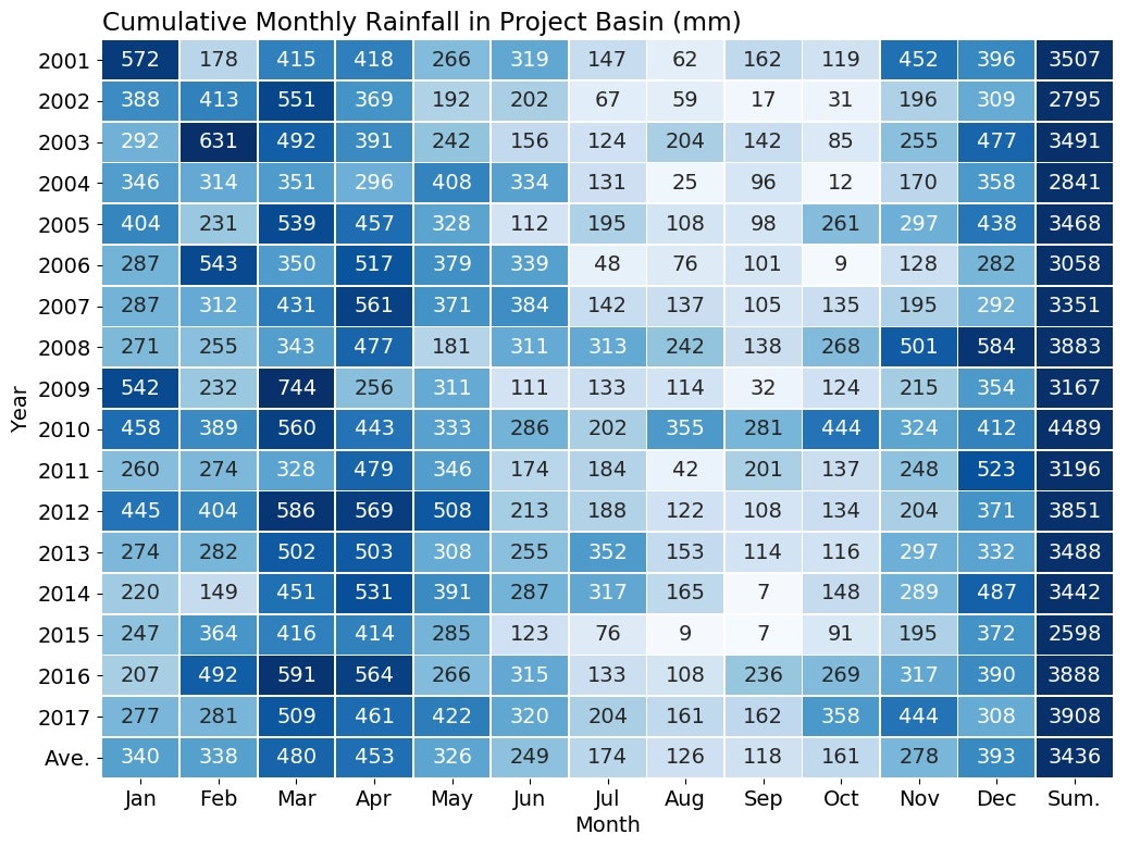
雨量データ表示プログラム
雨量の場合は、月平均・年平均よりは月別総計・年総計が知りたいので、流量表示プログラムに対し若干の変更を加えている。
# Outline of rainfall data
import numpy as np
import pandas as pd
import datetime
import matplotlib.pyplot as plt
import seaborn as sns


# global
_ylist=np.arange(2001,2018,1)
ylist=[]
for y in _ylist:
    ylist=ylist+[str(y)]


def rdata():
    df = pd.read_csv('data_df.csv', header=0, index_col=0)
    df.index = pd.to_datetime(df.index, format='%Y-%m-%d')
    df=df[df.index >= '2001-01-01']
    q=np.array(df['Dam'])
    ii=np.where(q<0)
    q[ii]=0
    d= df.index
    qq=pd.Series(np.array(q),index=d)
    return qq


def makedf(qq):
    mlist=['-01','-02','-03','-04','-05','-06','-07','-08','-09','-10','-11','-12']
    n=len(ylist)
    m=len(mlist)
    qt=np.zeros((n+1,m+1),dtype=np.float64) # sum of discharges of a month
    ct=np.zeros((n+1,m+1),dtype=np.int)     # sum of days of a manth
    for i,sy in enumerate(ylist): # year
        for j,sm in enumerate(mlist): # month
            sym=sy+sm
            qd=np.array(qq[sym])
            ii=np.where(0<=qd)
            qt[i,j]=np.sum(qd[ii])
            ct[i,j]=len(qd[ii])
    for i in range(n):
        qt[i,m]=np.sum(qt[i,0:m])
        ct[i,m]=np.sum(ct[i,0:m])
    for j in range(m):
        ct[n,j]=np.sum(ct[0:n,j])
        qt[n,j]=np.sum(qt[0:n,j])/len(ylist)
    qt[n,m]=np.sum(qt[0:n,0:m])/len(ylist)
    ct[n,m]=np.sum(ct[0:n,0:m])
    dfq = pd.DataFrame({'Year': ylist+['Ave.'],
                       'Jan' : qt[:,0],
                       'Feb' : qt[:,1],
                       'Mar' : qt[:,2],
                       'Apr' : qt[:,3],
                       'May' : qt[:,4],
                       'Jun' : qt[:,5],
                       'Jul' : qt[:,6],
                       'Aug' : qt[:,7],
                       'Sep' : qt[:,8],
                       'Oct' : qt[:,9],
                       'Nov' : qt[:,10],
                       'Dec' : qt[:,11],
                       'Sum.': qt[:,12]})
    dfq=dfq.set_index('Year')
    dfc = pd.DataFrame({'Year': ylist+['Sum'],
                       'Jan' : ct[:,0],
                       'Feb' : ct[:,1],
                       'Mar' : ct[:,2],
                       'Apr' : ct[:,3],
                       'May' : ct[:,4],
                       'Jun' : ct[:,5],
                       'Jul' : ct[:,6],
                       'Aug' : ct[:,7],
                       'Sep' : ct[:,8],
                       'Oct' : ct[:,9],
                       'Nov' : ct[:,10],
                       'Dec' : ct[:,11],
                       'Sum' : ct[:,12]})
    dfc=dfc.set_index('Year')
    return dfq,dfc


def fighmap1(dfq):
    wid=0.5*(len(ylist)+1)
    fsz=14
    plt.figure(figsize=(12,wid),facecolor='w')
    plt.rcParams['font.size']=fsz
    plt.rcParams['font.family']='sans-serif'
#    cm='YlGnBu'
    cm='Blues'
    sns.heatmap(dfq,annot=True,fmt='.0f',vmin=0,vmax=600,cmap=cm,cbar=False,linewidths=0.5)
    plt.xlabel('Month')
    plt.ylabel('Year')
    plt.yticks(rotation=0)
    plt.title('Cumulative Monthly Rainfall in Project Basin (mm)',loc='left')
    fnameF='fig_rf_hmap1.jpg'
    plt.savefig(fnameF, dpi=100, bbox_inches="tight", pad_inches=0.1)
    plt.show()


def fighmap2(dfc):
    wid=0.5*(len(ylist)+1)
    fsz=14
    plt.figure(figsize=(12,wid),facecolor='w')
    plt.rcParams['font.size']=fsz
    plt.rcParams['font.family']='sans-serif'
#    cm='YlGnBu'
    sns.heatmap(dfc,annot=True,fmt='5d',vmin=0,vmax=30,cbar=False,linewidths=0.5)
    plt.xlabel('Month')
    plt.ylabel('Year')
    plt.yticks(rotation=0)
    plt.title('Number of Monthly Available Values (days)',loc='left')
    fnameF='fig_rf_hmap2.jpg'
    plt.savefig(fnameF, dpi=100, bbox_inches="tight", pad_inches=0.1)
    plt.show()


def figts(df):
    # arrange of subplot
    # ------------------------------------
    # i= 0  i= 1  i= 2  i= 3  i= 4
    # i= 5  i= 6  i= 7  i= 8  i= 9
    # i=10  i=11  i=12  i=13  i=14
    # i=15  i=16
    # ------------------------------------
    icol=5
    irow=4
    fsz=11
    xmin=0;xmax=12
    ymin=0;ymax=1000
    x=np.array([1,2,3,4,5,6,7,8,9,10,11,12])
    x=x-0.5
    mlist=['Jan','Feb','Mar','Apr','May','Jun','Jul','Aug','Sep','Oct','Nov','Dec']
    emp=['']*12
    plt.figure(figsize=(12,12/icol*irow),facecolor='w')
    plt.rcParams['font.size']=fsz
    plt.rcParams['font.family']='sans-serif'
    plt.suptitle('Cumulative Monthly Rainfall in Project basin in Each Year', x=0.5,y=0.91,fontsize=fsz+4)
    plt.subplots_adjust(wspace=0.07,hspace=0.07)
    for i,sy in enumerate(ylist):
        num=i+1
        plt.subplot(irow,icol,num)
        plt.xlim([xmin,xmax])
        plt.ylim([ymin,ymax])
        if i==0 or i==5 or i==10 or i==15:
            plt.ylabel('Rainfall (mm/Month)')
        else:
            plt.yticks([])
        if i==12 or i==13 or i==14 or i==15 or i==16:
            plt.xticks(x,mlist,rotation=90)
        else:
            plt.xticks(x,emp,rotation=90)
        y=df.loc[sy][0:12]
        qa=df.loc[sy][12]
        plt.plot(x,y,'o-',color='#000080',lw=1)
        plt.plot([xmin,xmax],[qa/12,qa/12],'--',color='#ff0000',lw=2)
        plt.text(8.5,qa/12,'ave',fontsize=fsz,va='bottom',ha='center', color='#ff0000')
        s1='Year: '+sy
        s2='Sum: {0:.0f}'.format(qa)
        textstr=s1+'\n'+s2
        props = dict(boxstyle='square', facecolor='#ffffff', alpha=1)
        xs=xmin+0.05*(xmax-xmin); ys=ymin+0.95*(ymax-ymin)
        plt.text(xs,ys, textstr, fontsize=fsz,va='top',ha='left', bbox=props)
    fnameF='fig_rf3.jpg'
    plt.savefig(fnameF, dpi=100, bbox_inches="tight", pad_inches=0.1)
    plt.show()


def main():
    qq=rdata()
    dfq,dfc=makedf(qq)
    pd.options.display.precision = 0
    pd.set_option("display.width", 200)
    print(dfq)
    fighmap1(dfq)
    fighmap2(dfc)
    figts(dfq)


# ==============
# Execution
# ==============
if __name__ == '__main__': main()
画像事例(有効日ヒートマップは流量の場合と同じなので省略)
以 上