はじめに
2次元非定常熱伝導解析プログラムを改造して,1次元非定常熱伝導解析プログラムを作ってみました.
実務上,1次元でかまわないのですが,コンクリートの打継を考慮(上に打足していく)したときの温度分布を知りたいことがあるのですが,それを簡易に行うためのものです.
このプログラムの特徴というか難点は特に以下の2点でしょうか.
- 要素分割を細かくしないと精度がでないこと(出力事例で示しています)
- 温度固定境界が扱えないこと.ただしこの問題については,大きな熱伝達率と熱伝達境界外部温度を入力することで,近似的に温度指定境界を模擬できるので,実務上対応可能と考えています.
プログラム及び入力データ例
| プログラム | 説明 |
|---|---|
| py_fem_1Dheat.py | 1次元非定常熱伝導解析プログラム |
| inp_20L1.txt | 20要素モデルデータ |
| inp_40L1.txt | 40要素モデルデータ |
| inp_100L1.txt | 100要素モデルデータ |
| inp_2L2.txt | 熱伝達境界外部温度履歴データ |
| py_fig_1Dheat.py | 温度時刻歴作図プログラム |
| py_data1.py | モデルデータ作成プログラム |
| py_data2.py | 温度履歴データ作成プログラム |
1次元非定常熱伝導解析解説
非定常有限要素式の解法
2次元非定常熱伝導解析と同様,Crank-Nicolson 差分式に有限要素式を当てはめた結果は,以下のとおりです.
$$
\left(\frac{1}{2}[\boldsymbol{K}]+\frac{1}{\Delta t}[\boldsymbol{C}]\right){\boldsymbol{\Phi}(t+\Delta t)}
=\left(-\frac{1}{2}[\boldsymbol{K}]+\frac{1}{\Delta t}[\boldsymbol{C}]\right){\boldsymbol{\Phi}(t)}+\frac{{\boldsymbol{F}(t+\Delta t)}+{\boldsymbol{F}(t)}}{2}
$$
| $[\boldsymbol{K}]$ | :熱伝導マトリックス | $[\boldsymbol{C}]$ | :熱容量マトリックス |
| $\{\boldsymbol{\Phi}\}$ | :節点温度ベクトル | $\{\boldsymbol{F}\}$ | :熱流束ベクトル |
それぞれのマトリックス・ベクトルを,要素単位で示すと以下の通りとなります.
$$
\begin{align}
&[\boldsymbol{k}]=\cfrac{\kappa\cdot A}{\ell}
\begin{bmatrix}
1 & -1 \
-1 & 1
\end{bmatrix}
+\alpha_{ci}\cdot A
\begin{bmatrix}
1 & 0 \
0 & 0
\end{bmatrix}
+\alpha_{cj}\cdot A
\begin{bmatrix}
0 & 0 \
0 & 1
\end{bmatrix}
\
&[\boldsymbol{c}]=\rho \cdot c \cdot \ell \cdot A
\begin{bmatrix}
1/3 & 1/6 \
1/6 & 1/3
\end{bmatrix}
\
&{\boldsymbol{f}}=\cfrac{\dot{Q}\cdot\ell\cdot A}{2} \begin{Bmatrix} 1 \\ 1 \end{Bmatrix}
+\alpha_{ci}\cdot T_{ci}\cdot A \begin{Bmatrix} 1 \\ 0 \end{Bmatrix}
+\alpha_{cj}\cdot T_{cj}\cdot A \begin{Bmatrix} 0 \\ 1 \end{Bmatrix}
\end{align}
$$
| $\kappa$ | :要素熱伝導率 | $c$ | :要素比熱 | $\rho$ | :要素密度 |
| $\ell$ | :要素長 | $A$ | :要素断面積 | $\dot{Q}$ | :要素発熱率 |
| $\alpha_{ci}$ | :節点$i$の熱伝達率(熱伝達境界でなければ$\alpha_{ci}=0$) | ||||
| $\alpha_{ci}$ | :節点$j$の熱伝達率(熱伝達境界でなければ$\alpha_{cj}=0$) | ||||
| $T_i$ | :節点$i$の熱伝達境界外部温度 | ||||
| $T_j$ | :節点$i$の熱伝達境界外部温度 | ||||
発熱体に関する説明
セメント・コンクリートをモデルとした発熱体を扱えます.セメント.コンクリートの断熱温度上昇量を,以下の式で仮定します.
$$
T=K\cdot(1-e^{-\alpha\cdot t})
$$
| $T$: 断熱温度上昇量 | $K$: 最高上昇温度 | $\alpha$: 発熱速度を示すパラメータ | $t$: 時間 |
上式の中の,$K$ (Tk) および $\alpha$ (Al) を材料特性として入力します.
上式を用い,発熱量 $Q$ および発熱率 $\dot{Q}$ は以下のように表現できます.
$$
Q=\rho \cdot c \cdot T(t) \quad \rightarrow \quad \dot{Q}=\rho \cdot c \cdot T_k \cdot \alpha \cdot e^{-\alpha t}
$$
1次元非定常熱伝導解析プログラム
プログラム概要
- このプログラムは,1次元非定常熱伝導解析を行うものです.定常熱伝導問題には対応していません.
- 1次元ですが,コンクリートの打継(複数リフトの打設)を,打設時刻とその時点で有効な要素を指定することにより.自動的に考慮できます.
- 座標系においては,x方向が上向きと仮定しています
- 1次元解析ですので,要素側面は全て断熱条件であり,領域の下面と上面のみ,境界条件が考慮できます.
- 領域上下面の境界条件として,断熱境界,熱伝達境界が考慮できます.
- セメント・コンクリートをモデルとした発熱体を扱うことができます.
- 要素として,1要素2節点,1節点1自由度(温度あるいは熱流束)を有する線形要素が用いられています.
- 時間軸の離散化には,Crank-Nicolson 法が用いられています.
- 入力データファイル,出力データファイルは,空白区切りで記載される必要があり,ファイル名はコマンドライン引数として入力します.
- 入力データファイルには,モデル領域を定義するものと,熱伝達境界外部温度の履歴を定義するものの,2種類が必要です.
- 出力事例でも示しますが,このプログラムでは,要素分割を細かくしないと精度は出ません.
| 扱える境界条件 | |
|---|---|
| 項目 | 説明 |
| 断熱境界 | モデル領域の定義ファイルでモデル下端および上端の条件を指定します. |
| 熱伝達境界 | モデル領域の定義フィルで熱伝達率を指定します.また別ファイルでモデル下端および上端の熱伝達境界の外部温度履歴を指定します. |
温度指定境界について
このプログラムでは,温度指定境界は扱えません.温度固定の条件で連立方程式を処理して計算してみましたが,予想に反する答えしか出てこず,改善策が見つかっていません.
しかしながら,工学的には,大きな熱伝達率を入力し外部温度を設定すれば,近似的に温度固定境界と同等の条件を再現することができます.
FEM解析実行用スクリプト
python py_fem_1Dheat.py inp1.txt inp2.txt out.txt
| inp1.txt | : 解析モデルデータ入力ファイル(空白区切りデータ) |
| inp2.txt | : 熱伝達境界外部温度の履歴入力ファイル(空白区切りデータ) |
| out.txt | : 出力データファイル(空白区切りデータ) |
入力データ書式
解析モデルデータ
npoin  nele  nsec  koB  koT  delta  nlift  # Basic values for analysis
Ak  Ac  Arho  Tk  Al  AA                   # Material properties
     ..... (1 to nsec) .....               #
tlift_1  tlift_2  .... (1 line input) .... # Placing time of each lift
alphac_B  alphac_T                         # Heat transfer rates of bottom and top
node-1  node-2  isec  lift                 # Element connectivity, Material set number, lift number
     ..... (1 to nele) .....               #   (counterclockwise order of node numbers)
x  T0                                      # Coordinates of node, initial temperature of node
     ..... (1 to npoin) .....              #
n1out                                 # Number of nodes for output of temperature time history
n1node_1  ..... (1 line input) .....  # Node number for above
n2out                                 # frequency of output of temperatures of all nodes
n2step_1  ..... (1 line input) .....  # Time step number for above (Omit data input if ntout=0)
| npoin, nele, nsec | : 節点数,要素数,材料特性数 |
| koB | : 下端境界条件(0:断熱,1:熱伝達) |
| koT | : 上端境界条件(0:断熱,1:熱伝達) |
| delta | : 計算時間間隔 |
| nlift | : 打設リフト数 |
| Ak, Ac, Arho | : 熱伝導率,比熱,密度 |
| Tk, Al, AA | : 最高断熱上昇温度,発熱速度パラメータ,要素断面積 |
| x, T0 | : 節点座標,節点初期温度 |
| n1out | : 全時刻歴を出力する節点数 |
| n1node | : 全時刻歴を出力する節点番号 |
| n2out | : 全節点温度を出力する時間ステップ数 |
| n2step | : 全節点温度を出力する時間ステップ番号 |
熱伝達境界外部温度の履歴
空白区切りで,3列の数値の入力が必須です.たとえ熱伝達境界でなくても0などの適当な数値を入力しておきます.
 0   TcinB[0]  TcinT[0]
 1   TcinB[1]  TcinT[1]
 2   TcinB[2]  TcinT[2]
 ..  ........  ........
 i   TcinB[i]  TcinT[i]
 ..  ........  ........
 .... (until end of calculation time) ....
| TcinB | : 下端熱伝達境界外部温度履歴 |
| TcinT | : 上端熱伝達境界外部温度履歴 |
出力データ書式
npoin  nele  nsec  koB  koT  delta  nlift  niii  n1out  n2out
    (Each value of above)
sec  Ak  Ac  Arho  Tk  Al  AA
    sec  : Material number
    Ak   : Heat conductivity coefficient
    Ac   : Specific heat
    Arho : Unit weight
    Tk   : Maximum temperature rize
    Al   : Heat release rate
    AA   : Section area of element
    ..... (1 to nsec) .....
node  x  tempe0  alphac
    node   : Node number
    x      : x-ccordinate
    tempe0 : Initial temperature
    alphac : Heat transfer rate of bottom and top node
    ..... (1 to npoin) .....
elem  i  j  sec  lift  time
    elem : Element number
    i    : Node number of start point
    j    : Node number of second point
    sec  : Material number
    lift : Lift number
    time : Placing time of lift
    ..... (1 to nele) .....
iii  ttime  Node_(xx)  Node_(xx)  Node_(xx) .....
    iii       : Time step
    ttime     : Time
    Node-(xx) : Node number
    Time historis of each node temperature are written.
    ..... (0 to end of calculation time) .....
node  t=0.0  t=(xx)  t=(xx)0  t=(xx) .....
    node   : Node number
    t=(xx) : Specified time
    Node temperatures at specified time are written.
    ..... (1 to npoin) .....
n=(total degrees of freedom)  time=(calculation time)
出力事例
モデル概要
高さ10mの既設のコンクリートブロックの上に,1リフト高2mのコンクリートを5リフト打ち上げた場合の温度履歴を計算します.既設コンクリートは発熱は終わっており,初期温度は下端で10度,表面で20度に設定しています.新規打設コンクリートは,打設温度30度でリフト表面は熱伝達境界(熱伝達率10 kcal/m$^2$ h $^{\circ}$C)とし,外部温度は20度に設定しています.
既設コンクリート下端は,近似的に温度固定境界とするため,熱伝達率を10000 kcal/m$^2$ h $^{\circ}$Cと大きくとっています.
| Characteristics of model | |
|---|---|
| Heat conductivity coefficient | 2.5 kcal/m h $^{\circ}$C |
| Specific heat | 0.28 kcal/kg $^{\circ}$C |
| Unit weight | 2350 kg/m$^3$ |
| Adiabatic temperature raise for new concrete |
$T=K\cdot(1-e^{-\alpha t})$, K=40$^{\circ}$C, α=0.2, t: hour |
| Element section area | 1m$^2$ |
| Model | Total length: 20m Old concrete: 10m New concrete: 10m, 5 lifts with height of 2m, Placing interval: 3 days (72 hours) |
| Conditions for analysis | |
|---|---|
| New concrete placing temperature | 30 $^{\circ}$C |
| Old concrete initial temperature | from 10 $^{\circ}$C at bottom to 20 $^{\circ}$C at surface |
| Boundary condition of bottom | Temperature fixed with outside temperature 10 $^{\circ}$c (approximately) Heat transfer rate of bottom boundary: 10000 kcal/m$^2$ h $^{\circ}$C |
| Boundary condition of top | Heat transfer boundary with outside temperature of 20 $^{\circ}$C Heat transfer rate of top boundary: 10 kcal/m$^2$ h $^{\circ}$C |
| Time increment for analysis | 0.1 hour |
FEM解析実行用スクリプト
python py_fem_1Dheat.py inp_100L1.txt inp_2L2.txt out_100L.txt
python py_fem_1Dheat.py inp_40L1.txt inp_2L2.txt out_40L.txt
python py_fem_1Dheat.py inp_20L1.txt inp_2L2.txt out_20L.txt
| inp_100L1.txt | : 解析モデルデータ入力ファイル(空白区切りデータ,100要素) |
| inp_40L1.txt | : 解析モデルデータ入力ファイル(空白区切りデータ,40要素) |
| inp_20L1.txt | : 解析モデルデータ入力ファイル(空白区切りデータ,20要素) |
| inp_2L2.txt | : 熱伝達境界外部温度の履歴入力ファイル(空白区切りデータ) |
| out_1D.txt | : FEM解析出力データファイル(空白区切りデータ) |
温度履歴作図プログラム実行用スクリプト
python py_fig_1Dheat.py out_100L.txt
cp _fig_tem_his.png fig_his_100.png

python py_fig_1Dheat.py out_40L.txt
cp _fig_tem_his.png fig_his_040.png

python py_fig_1Dheat.py out_20L.txt
cp _fig_tem_his.png fig_his_020.png
このプログラムでは,_fig_tem_his.png という画像ファイルが自動的に作成されます.
節点温度履歴図出力事例
プログラム:py_fig_1Dheat.py を用い matplotlib で作成した png 画像です.
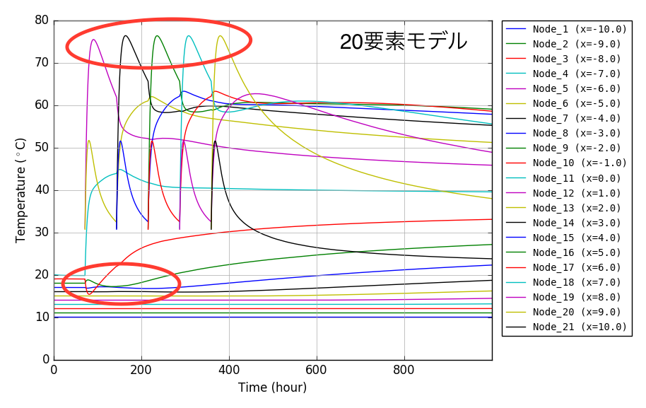
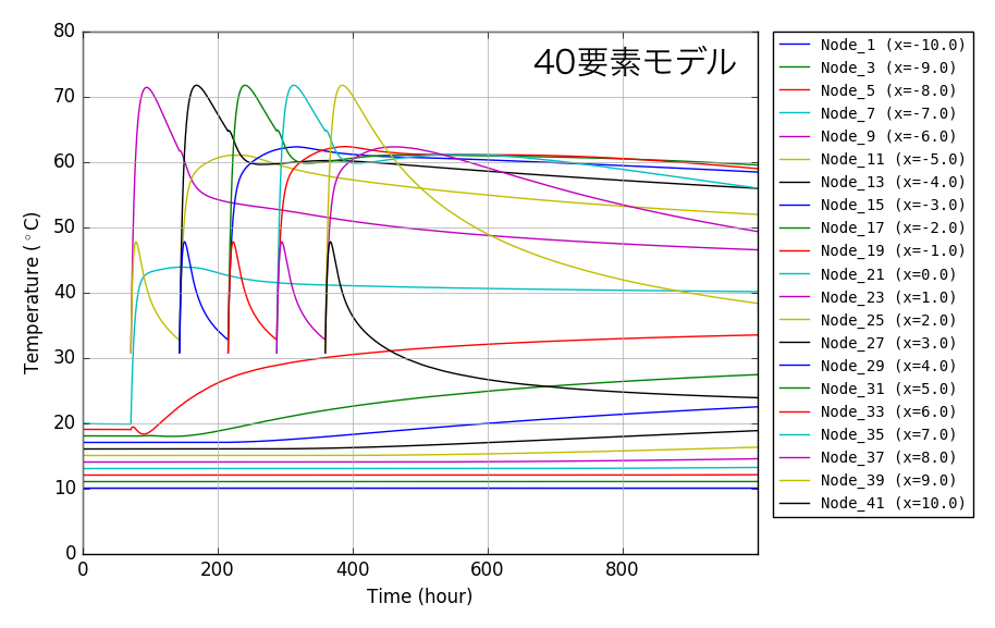
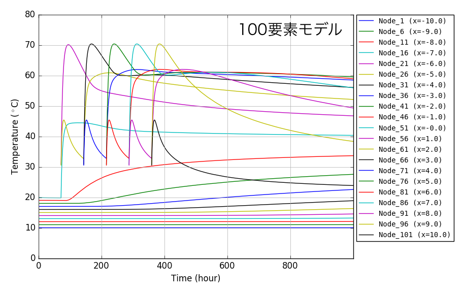
下に要素分割を20,40,100とした事例を示します.
要素分割20では何かがおかしい!赤い楕円で囲まれた部分に着目してみると,以下のことに気が付くと思います.
- 打設温度30度,断熱温度上昇量40度のコンクリートなのに最高温度が75度以上まで上がっている.
- 新コンクリートとの境界付近の旧コンクリートにおいて,1リフト打設直後にあり得ない温度履歴となっている.
上記現象は,要素数の増加に伴い改善されていることがわかります.
以 上