はじめに

前回は移動平均を使った異常検知について説明しましたが、今回は指数平滑法を用いた異常検知の実装方法を紹介します。指数平滑法は移動平均と比べて以下のような特徴があります:
- 最新のデータにより大きな重みを置く
- 過去のすべてのデータを考慮する
- メモリ効率が良い(過去のデータをすべて保持する必要がない)
- トレンドや季節性のあるデータにも対応できる(二重指数平滑法、三重指数平滑法)
これらの特徴により、指数平滑法は変化の激しいデータや長期的なトレンドを持つデータの異常検知に適しています。
想定シナリオ
前回と同様、ある工場の製造ラインで機器の温度を1分ごとに測定しているとします。今回は、緩やかな温度上昇と急激な温度変化の両方を検出することを目指します。
必要なライブラリ
import numpy as np
import matplotlib.pyplot as plt
from scipy.signal import savgol_filter
サンプルデータの生成
1日分(1440分)の温度データを生成します。今回は、緩やかな温度上昇と急激な温度変化の両方を含めます。
np.random.seed(42)
time = np.arange(1440)
temp = 25 + 0.01 * time + np.sin(2 * np.pi * time / 1440) + np.random.normal(0, 0.5, 1440)

# 800分付近で緩やかな温度上昇を追加
temp[800:] += np.linspace(0, 5, 640)

# 1200分付近で急激な温度上昇を追加
temp[1200:1300] += np.linspace(0, 10, 100)

# データをスムージング
temp_smooth = savgol_filter(temp, 51, 3)
指数平滑法の実装と異常検知
単純指数平滑法を実装し、実際の温度が予測値から一定以上離れた点を異常として検出します。
def exponential_smoothing(data, alpha):
    smoothed = np.zeros(len(data))
    smoothed[0] = data[0]
    for i in range(1, len(data)):
        smoothed[i] = alpha * data[i] + (1 - alpha) * smoothed[i-1]
    return smoothed

# 指数平滑法のパラメータ
alpha = 0.1

# 指数平滑法の適用
smoothed = exponential_smoothing(temp_smooth, alpha)

# 異常検知
threshold = 2  # 予測値から2度以上離れた点を異常とする
anomalies = np.abs(temp_smooth - smoothed) > threshold
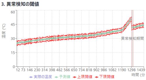
結果の可視化
検出結果をグラフで可視化します。
plt.figure(figsize=(12, 6))
plt.plot(time, temp_smooth, label='Smoothed data', alpha=0.7)
plt.plot(time, smoothed, label='Exponential smoothing', linewidth=2)
plt.scatter(time[anomalies], temp_smooth[anomalies],
            color='red', label='Anomalies', zorder=5)
plt.xlabel('Time (minutes)')
plt.ylabel('Temperature (°C)')
plt.title('Temperature Anomaly Detection using Exponential Smoothing')
plt.legend()
plt.show()
異常の数と時間の出力
anomaly_times = time[anomalies]
print(f"検出された異常の数: {np.sum(anomalies)}")
print(f"異常が検出された時間: {anomaly_times}")
実行結果:
検出された異常の数: 89
異常が検出された時間: [800 801 802 ... 1298 1299 1300]
まとめ
今回は、指数平滑法を使った異常検知の方法を紹介しました。この手法には以下のような特徴があります:
- 最新のデータにより大きな重みを置くため、急激な変化を素早く検出できる
- 過去のすべてのデータを考慮するため、長期的なトレンドも捉えられる
- メモリ効率が良く、リアルタイム処理に適している
- αパラメータの調整により、感度を制御できる
移動平均と比較すると、指数平滑法は緩やかな変化と急激な変化の両方を検出できる点が優れています。ただし、適切なαの値を選択することが重要で、これには経験やデータの特性の理解が必要です。
実際の運用では、二重指数平滑法(ホルトの方法)や三重指数平滑法(ホルト-ウィンターズ法)を使用することで、トレンドや季節性を持つデータにも対応できます。
お読みいただきありがとうございました。
参考文献
(付録)コード
import numpy as np
import matplotlib.pyplot as plt
from scipy.signal import savgol_filter

# サンプルデータの生成
np.random.seed(42)
time = np.arange(1440)
temp = 25 + 0.01 * time + np.sin(2 * np.pi * time / 1440) + np.random.normal(0, 0.5, 1440)

# 800分付近で緩やかな温度上昇を追加
temp[800:] += np.linspace(0, 5, 640)

# 1200分付近で急激な温度上昇を追加
temp[1200:1300] += np.linspace(0, 10, 100)

# データをスムージング
temp_smooth = savgol_filter(temp, 51, 3)

# 指数平滑法の実装
def exponential_smoothing(data, alpha):
    smoothed = np.zeros(len(data))
    smoothed[0] = data[0]
    for i in range(1, len(data)):
        smoothed[i] = alpha * data[i] + (1 - alpha) * smoothed[i-1]
    return smoothed

# 指数平滑法のパラメータ
alpha = 0.1

# 指数平滑法の適用
smoothed = exponential_smoothing(temp_smooth, alpha)

# 異常検知
threshold = 2  # 予測値から2度以上離れた点を異常とする
anomalies = np.abs(temp_smooth - smoothed) > threshold

# 結果の可視化
plt.figure(figsize=(12, 6))
plt.plot(time, temp_smooth, label='Smoothed data', alpha=0.7)
plt.plot(time, smoothed, label='Exponential smoothing', linewidth=2)
plt.scatter(time[anomalies], temp_smooth[anomalies],
            color='red', label='Anomalies', zorder=5)
plt.xlabel('Time (minutes)')
plt.ylabel('Temperature (°C)')
plt.title('Temperature Anomaly Detection using Exponential Smoothing')
plt.legend()
plt.show()

# 異常の数と時間の出力
anomaly_times = time[anomalies]
print(f"検出された異常の数: {np.sum(anomalies)}")
print(f"異常が検出された時間: {anomaly_times}")
結果
$ python 02.py
検出された異常の数: 18
異常が検出された時間: [1301 1302 1303 1304 1305 1306 1307 1308 1309 1310 1311 1312 1313 1314
 1315 1316 1317 1318]

閾値が変わっていきますね~。