BoTorchでLCBを自作して試してみました.
ベイズ最適化における獲得関数
ベイズ最適化では, 次に観測する候補点を以下のように獲得関数$\mathcal{A}(\boldsymbol{x})$の最大化に基づいて決定します.
\boldsymbol{x}^* = \arg\max_{\boldsymbol{x}}\mathcal{A}(\boldsymbol{x})
活用と探索のトレードオフをうまく汲み取った獲得関数を設計し, なるべく少ない回数で最適解を見つけることが目的です.
BoTorchでの実装方法
BoTorchには解析計算による獲得関数とモンテカルロ獲得関数の2種類があります.
BoTorchの獲得関数の基底クラスはいくつかありますが, 今回はAnalyticAcquisitionFunctionを基底クラスに利用した解析計算による獲得関数を実装する方法を試してみます.
大まかな内容としては以下になります
from torch import Tensor
from botorch.models.model import Model
from botorch.acquisition.objective import PosteriorTransform
from botorch.acquisition.analytic import AnalyticAcquisitionFunction

class MyAcquFunc(AnalyticAcquisitionFunction):
    """
    自作獲得関数
    """

    def __init__(
        self,
        model: Model,
        posterior_transform: Optional[PosteriorTransform] = None
    ):
        super().__init__(model=model, posterior_transform=posterior_transform)
        # TODO: 追加で定義するものがあれば実装

    def forward(self, X: Tensor) -> Tensor:
        """
                候補点の獲得関数の値を返す.
        Args:
            X (Tensor): 候補点
        """
        # TODO: 候補点Xの獲得関数の値を返す
ExpectedImprovementの実装確認
Expected Implovementは改善量の期待値を返す獲得関数です.
BoTorchで既にExpectedImprovementとして実装されているので, その実装を見てみます.
class ExpectedImprovement(AnalyticAcquisitionFunction):
    r"""Single-outcome Expected Improvement (analytic).

    Computes classic Expected Improvement over the current best observed value,
    using the analytic formula for a Normal posterior distribution. Unlike the
    MC-based acquisition functions, this relies on the posterior at single test
    point being Gaussian (and require the posterior to implement `mean` and
    `variance` properties). Only supports the case of `q=1`. The model must be
    single-outcome.

    `EI(x) = E(max(f(x) - best_f, 0)),`

    where the expectation is taken over the value of stochastic function `f` at `x`.

    Example:
        >>> model = SingleTaskGP(train_X, train_Y)
        >>> EI = ExpectedImprovement(model, best_f=0.2)
        >>> ei = EI(test_X)

    NOTE: It is *strongly* recommended to use LogExpectedImprovement instead of regular
    EI, because it solves the vanishing gradient problem by taking special care of
    numerical computations and can lead to substantially improved BO performance.
    """

    def __init__(
        self,
        model: Model,
        best_f: Union[float, Tensor],
        posterior_transform: Optional[PosteriorTransform] = None,
        maximize: bool = True,
    ):
        r"""Single-outcome Expected Improvement (analytic).

        Args:
            model: A fitted single-outcome model.
            best_f: Either a scalar or a `b`-dim Tensor (batch mode) representing
                the best function value observed so far (assumed noiseless).
            posterior_transform: A PosteriorTransform. If using a multi-output model,
                a PosteriorTransform that transforms the multi-output posterior into a
                single-output posterior is required.
            maximize: If True, consider the problem a maximization problem.
        """
        super().__init__(model=model, posterior_transform=posterior_transform)
        self.register_buffer("best_f", torch.as_tensor(best_f))
        self.maximize = maximize

    @t_batch_mode_transform(expected_q=1)
    def forward(self, X: Tensor) -> Tensor:
        r"""Evaluate Expected Improvement on the candidate set X.

        Args:
            X: A `(b1 x ... bk) x 1 x d`-dim batched tensor of `d`-dim design points.
                Expected Improvement is computed for each point individually,
                i.e., what is considered are the marginal posteriors, not the
                joint.

        Returns:
            A `(b1 x ... bk)`-dim tensor of Expected Improvement values at the
            given design points `X`.
        """
        mean, sigma = self._mean_and_sigma(X)
        u = _scaled_improvement(mean, sigma, self.best_f, self.maximize)
        return sigma * _ei_helper(u)
self._mean_and_sigma(基底クラスAnalyticAcquisitionFunctionのメソッド)の部分で事後分布の平均と分散を取得します.
_scaled_improvementで改善量$I(x)$を求めています
I(x) = \left\{
\begin{array}{ll}
\frac{f(x) - f_{\rm best}}{\sigma^2} & 最大化の場合 \\
\frac{f_{\rm best} - f(x)}{\sigma^2} & 最小化の場合
\end{array}
\right.
実装としては以下のようになっています。
def _scaled_improvement(
    mean: Tensor, sigma: Tensor, best_f: Tensor, maximize: bool
) -> Tensor:
    """Returns `u = (mean - best_f) / sigma`, -u if maximize == True."""
    u = (mean - best_f) / sigma
    return u if maximize else -u
上記で取得した改善量の期待値を計算して返しています.
def _ei_helper(u: Tensor) -> Tensor:
    """Computes phi(u) + u * Phi(u), where phi and Phi are the standard normal
    pdf and cdf, respectively. This is used to compute Expected Improvement.
    """
    return phi(u) + u * Phi(u)
ここで, phi, Phiはそれぞれbotorch.utils.probability.utils.phiとbotorch.utils.probability.utils.ndtrで標準正規分布のpdfとcdfです。
($f(x)$は正規分布に従うので, $f(x) - f_{\rm best}$もまた正規分布に従います)
自作獲得関数を試す
今回はシンプルな獲得関数であるLower Confidence Bound (LCB) を実装して試してみます.
{\rm LCB}(\boldsymbol{x}) = - (\mu(\boldsymbol{x}) - \beta\sigma(\boldsymbol{x}))
$\beta$はハイパーパラメータです.
上記は最小化探索の場合で, 最大化の場合は符号が反転します.
class LCB(AnalyticAcquisitionFunction):
    """
    Lower Confidence Bound
    """
    def __init__(
        self,
        model: Model,
        maximize: bool = True,
        beta: float = 0.5,
        posterior_transform = None
    ) -> None:
        super().__init__(model=model, posterior_transform=posterior_transform)
        self.beta = beta
        self.maximize = maximize

    def forward(self, X: torch.Tensor) -> torch.Tensor:
        mean, sigma = self._mean_and_sigma(X)
        lcb = - (mean - self.beta * torch.sqrt(sigma))
        if self.maximize:
            lcb = - lcb
        return lcb
自作したLCBを利用したoptimizerを実装しておきます
from botorch.models import SingleTaskGP
from gpytorch.mlls import ExactMarginalLogLikelihood
from botorch import fit_gpytorch_model
from botorch.utils.transforms import unnormalize, normalize
from botorch.models.transforms.outcome import Standardize
from botorch.optim import optimize_acqf


class BayesOptimizer:
    def __init__(self):
        self.model = None

    def fit_gp(self, X, y):
        """
        GPのフィッティング
        """
        self.model = SingleTaskGP(X, y, outcome_transform=Standardize(m=1))
        mll = ExactMarginalLogLikelihood(self.model.likelihood, self.model)
        fit_gpytorch_model(mll)
        posterior = self.model.posterior(
            X=X, posterior_transform=None
        )

    def get_candidates(self, X, y, maximize=True):
        """
        実験候補点取得.
        Xは0-1正規化されている想定
        """
        self.fit_gp(X, y)

        X_dim = X.size()[1]
        bounds = torch.zeros(2, X_dim)
        bounds[1] = 1
        beta = torch.log(torch.Tensor([X.size()[0]]))[0]  # LCBのハイパラ
        acq_func = LCB(model=self.model, maximize=maximize, beta=beta)  # 獲得関数に自作のLCBを利用
        candidates, acq_values = optimize_acqf(acq_func, bounds=bounds, q=1, num_restarts=10, raw_samples=100)
        return candidates.detach()
Branin functionの最小値を探索するシミュレーションをしてみます.
import random
from botorch.test_functions import Branin

problem = Branin()
bounds = problem.bounds
def branin(x):
    return torch.unsqueeze(problem(x), dim=1)

# 初期観測データを適当に生成
x_init = x_obj = torch.tensor([[-3, 1], [2.0, 10.0]]).double()
y_init = branin(x_init)

# LCBによる探索とランダム探索の比較シミュレーション
bo_xs = x_init
bo_ys = y_init
random_ys = y_init
best_bo = [torch.min(bo_ys)]
best_random = [torch.min(random_ys)]

# 探索開始
for i in range(20):
    # ベイズ最適化による探索候補取得
    optimizer = BayesOptimizer()
    bo_xs_norm = normalize(bo_xs, bounds)
    bo_x_candidates = optimizer.get_candidates(bo_xs_norm, bo_ys, maximize=False)
    bo_x_candidates = unnormalize(bo_x_candidates, bounds)
    # ランダム探索の候補取得
    x1 = random.uniform(bounds[0][0], bounds[1][0])
    x2 = random.uniform(bounds[0][1], bounds[1][1])
    random_x_candidates = torch.Tensor([[x1, x2]])
    # 候補点の観測
    bo_y_candidates = branin(bo_x_candidates)
    random_y_candidates = branin(random_x_candidates)
    # 観測データに追加
    bo_xs = torch.cat([bo_xs, bo_x_candidates])
    bo_ys = torch.cat([bo_ys, bo_y_candidates])
    random_ys = torch.cat([random_ys, random_y_candidates])
    best_bo.append(torch.min(bo_ys))
    best_random.append(torch.min(random_ys))
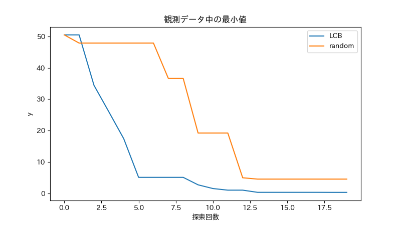
観測データ中の最小値の推移をプロットすると以下のようになりました. ランダム探索よりは効率よく探索できてることが確認できました.
(簡単な目的関数だったのでランダム探索でもそれなりに最小化できてしまいましたが...)
参考