はじめに
LDAを使って、高次元にベクトル化したPOSデータをクラスタリングできるという話。
クラスタの遷移とかも見てみた。
LDA
ニュース記事などをトピック別に分けたりするときに使うあれ。
次元削減手法の一つで、文書のモデル化に適した手法で、トピックモデルとかいうやつ。
いわゆるソフトクラスタリングができて、データは複数のクラスタに属することができる。(クラスタ1の所属確率0.8、クラスタ2の所属確率0.2、みたいな)
詳しくは、他の記事とか書籍とか調べれば出てくると思う。
POSデータへの適用
POSデータで商品ごとの購入回数や売り上げなどでユーザーをクラスタリングしたい場合、商品種類が多いと次元が多いデータになる。
それをkmeansのような距離を使う手法でクラスタリングする場合、次元が多いせいで計算の都合上距離が急速に大きくなってしまい、うまくクラスタリングすることができなくなってしまう。
一方LDAでは、例えば文書を分けるとき、BoW形式でベクトル化してモデルを適用したりするけど、単語数が膨大なのでかなり高次元なデータになるはず。つまりLDAのようなトピックモデルは高次元データでもクラスタリングしやすいというわけで、「おや?POSデータのクラスタリングとかにも向いてるんじゃね?」と思った。
使用データ
kaggleの「eCommerce purchase history from electronics store」を使う。(出典:https://rees46.com/)
2020年4月から2020年11月までの大型家電製品および電子機器のオンラインストア購入データ。
クラスタリング実行
LDAはソフトクラスタリングができるが、今回は所属確率が最も高いクラスタだけを見てハードクラスタリングとして扱う。
準備
まず必要なパッケージをimport。
# パッケージインポート
import numpy as np
import matplotlib as mpl
import matplotlib.pyplot as plt
import matplotlib.gridspec as gridspec
import seaborn as sns
import pandas as pd
import datetime as dt
import sklearn
from sklearn.preprocessing import MinMaxScaler
from sklearn.preprocessing import StandardScaler
from sklearn.cluster import KMeans
from sklearn.decomposition import LatentDirichletAllocation
import time
import os
import glob
import codecs
sns.set()
'''
numpy 1.18.1
matplotlib 3.1.3
seaborn 0.10.0
pandas 1.0.3
sklearn 0.22.1
'''
データの読み込みと加工と抽出。
file='kz.csv'
df = pd.read_csv(file, dtype={'user_id':str, 'order_id':str})
df=df[['event_time', 'category_code', 'brand', 'price', 'user_id', 'order_id']]
df=df.dropna()
df['event_time']=df['event_time'].str[:-4]
df['event_time']=pd.to_datetime(df['event_time'])
df=df[df['event_time']>=dt.datetime(2020,1,1)]
df=df.sort_values('event_time')
# ブランドとカテゴリーを結合する
df_cat_split=df['category_code'].str.split('.', expand=True)
df_cat_split.loc[(pd.isna(df_cat_split[2])), 2]=df_cat_split[1]
df_cat_split[3]=df_cat_split[1]+'.'+df_cat_split[2]
df['category']=df_cat_split[3].values
df['brand_category']=df['brand']+'.'+df['category']
# 各カラムのユニーク数
print('order_id', df['order_id'].unique().shape[0])
print('user_id', df['user_id'].unique().shape[0])
print('category_code', df['category_code'].unique().shape[0])
print('brand', df['brand'].unique().shape[0])
print('brand_category', df['brand_category'].unique().shape[0])
'''
order_id 331424
user_id 203235
category_code 123
brand 570
brand_category 1375
'''
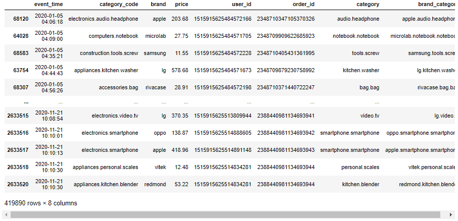
display(df)
データを前半と後半の二つに分ける。
# データを半分に分ける
df_before=df.iloc[:int(len(df)/2.),:]
df_after=df.iloc[int(len(df)/2.):,:]

# どちらのデータにも存在しているuser_idを抽出
df_target=pd.merge(df_before[['user_id']], df_after[['user_id']], on=['user_id'], how='inner')['user_id'].unique()
df_target=pd.DataFrame(df_target, columns=['user_id'])
# どちらのデータにも存在しているuser_idを対象にしたデータを作る
df_before=df_before[df_before['user_id'].isin(df_target['user_id'].values)]
df_after=df_after[df_after['user_id'].isin(df_target['user_id'].values)]
# 2つのデータの期間とuser_idのユニーク数を表示
print('before\n', df_before['event_time'].min())
print('', df_before['event_time'].max())
print('\nafter\n',df_after['event_time'].min())
print('', df_after['event_time'].max())
print('\nUnique User Cnt', len(df_target))
'''
before
 2020-01-05 04:35:21
 2020-08-14 08:58:58

after
 2020-08-14 08:59:17
 2020-11-21 09:59:55

Unique User Cnt 15527
'''
user_idごとの商品別購入金額のデータマートを作成。
価格が高いと購入のされやすさも変わると考え、重みをつけるという意味でも購入回数ではなく、購入金額のデータマートを作成した。
# ピボットでマートを作る
def df_pivot(df, index, columns, values, aggfunc):
df_mart=df.pivot_table(index=index, columns=columns, values=values, aggfunc=aggfunc).reset_index()
df_mart=df_mart.fillna(0)
return df_mart
# LDAに食わせる用の加工
def df_to_np(df_mart):
df_data=df_mart.copy().iloc[:,1:]
df_data = df_data.values
return df_data
row='user_id'
col='brand_category'
val='price'
df_mart=df_pivot(df_before, row, col, val, 'sum')
df_mart2=df_pivot(df_after, row, col, val, 'sum')
# df_martとdf_mart2で重複していないカラム名をとってくる
after=np.hstack((df_mart.columns.values, df_mart2.columns.values))
unique_after, counts_after = np.unique(after, return_counts=True)
non_dep_after=unique_after[counts_after == 1]
# さっきの重複していないカラム名の中で、df_martに入っていてdf_mart2に入っていないカラム名を抽出
before=np.hstack((non_dep_after, df_mart.columns.values))
unique_before, counts_before = np.unique(before, return_counts=True)
dep_before=unique_before[counts_before != 1]
# df_mart2にdf_mart固有のカラム名の列を追加
for col in dep_before:
df_mart2[col]=0.
# これでdf_martとdf_mart2のカラムがそろう
df_mart=df_mart[df_mart.columns]
df_mart2=df_mart2[df_mart.columns]
# LDAに食わせる用の加工
df_data=df_to_np(df_mart)
df_data2=df_to_np(df_mart2)
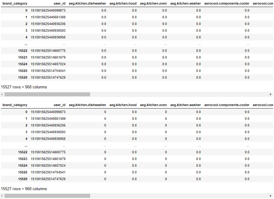
display(df_mart)
display(df_mart2)
display(df_data)
display(df_data2)


LDAでクラスタリング
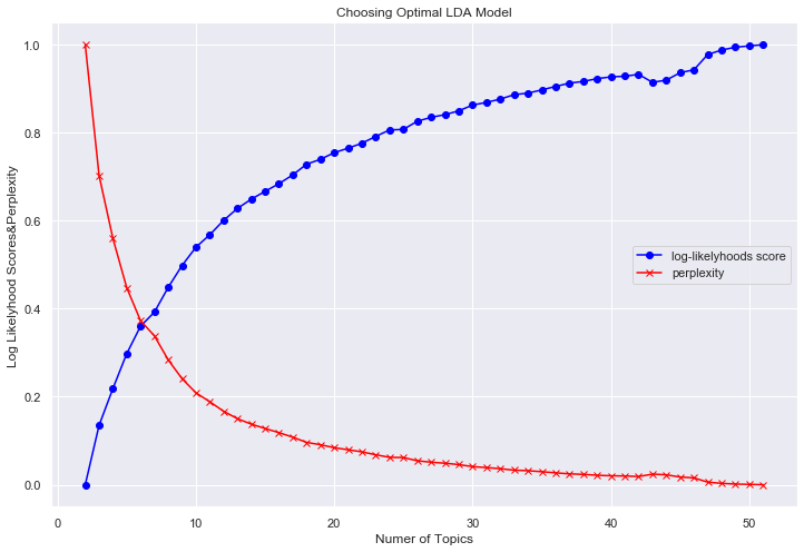
2~50のクラスタ(トピック)数のモデルを作る。
対数尤度(大きいほど良い)とperplexity(小さいほど良い)はクラスタ数が大きくなるほど良くなってしまったので、適当にクラスタ数=6に設定した。(クラスタ数ってどうやって決めるんだろ?)
# LDAのモデルを作る関数
def model_plot_opt(tfidf_data, topic_list, plot_enabled=True):
    # 定義
    n_topics = list(topic_list.astype(int))
    perplexities=[]
    log_likelyhoods_scores=[]
    models=[]
    search_params = {'n_components': n_topics}
    minmax_1 = MinMaxScaler()
    minmax_2 = MinMaxScaler()

    # 設定したトピック数ごとのモデルを作る
    for i in n_topics:
        print('topic_cnt:',i)
        lda = LatentDirichletAllocation(n_components=i,random_state=0,
                                        learning_method='batch',
                                        max_iter=25)
        lda.fit(tfidf_data)
        lda_perp = lda.perplexity(tfidf_data)
        log_likelyhoods_score = lda.score(df_data)
        perplexities.append(lda_perp)
        log_likelyhoods_scores.append(log_likelyhoods_score)
        models.append(lda)

    # 対数尤度とperplexityを正規化したものをプロット
    if plot_enabled:
        # 正規化
        log_likelyhoods_scores_std=minmax_1.fit_transform(np.array(log_likelyhoods_scores).reshape(len(log_likelyhoods_scores),1))
        perplexities_std=minmax_2.fit_transform(np.array(perplexities).reshape(len(perplexities),1))
        # 図作成
        plt.figure(figsize=(12, 8))
        ax=plt.subplot(1,1,1)
        ax.plot(n_topics, log_likelyhoods_scores_std, marker='o', color='blue', label='log-likelyhoods score')
        ax.set_title("Choosing Optimal LDA Model")
        ax.set_xlabel("Numer of Topics")
        ax.set_ylabel("Log Likelyhood Scores&Perplexity")
        ax.plot(n_topics, perplexities_std, marker='x', color='red', label='perplexity')
        plt.legend()
        plt.show()

    return models, log_likelyhoods_scores_std, perplexities_std

# モデルのリストと正規化した対数尤度とperplexityを定義
models_list, log_likelyhoods_scores_std, perplexities_std = model_plot_opt(df_data, np.linspace(2,51,50))
# 適当に6にする
lda=models_list[4]
print('topic_num:', lda.components_.shape[0])
'''
topic_num: 6
'''
各クラスタの特徴を見ていく。
まずは各クラスタにおける、商品の出現確率上位を抽出。
# 各トピックにおける、商品の出現確率上位20を取得する関数
def component(lda, features):
    df_component=pd.DataFrame()
    for tn in range(lda.components_.shape[0]):
        row = lda.components_[tn]
        words = [features[i] for i in row.argsort()[:-20-1:-1]]
        df_component[tn]=words
        words = ', '.join([features[i] for i in row.argsort()[:-20-1:-1]])
    return df_component

# 各トピックにおける、商品の出現確率上位5まで抽出
features = df_mart.iloc[:,1:].columns.values
df_component=component(lda, features)
display(df_component.iloc[:5,:])
(EXCELで体裁を整えた↓)

また、各クラスタにおける、商品の平均購入数を抽出。
# user_idごとの所属確率が最も高いトピックを列として追加したdfを作成
def create_topic_no(df_mart, df_data, lda):
df_id_cluster=df_mart[[row]]
df_topic=pd.DataFrame(lda.transform(df_data))
topic=df_topic.loc[:,:].idxmax(axis=1).values
df_id_cluster['topic']=topic
return df_id_cluster
df_id_cluster=create_topic_no(df_mart, df_data, lda)
df_id_cluster2=pd.merge(df_mart, df_id_cluster, on=['user_id'], how='left')
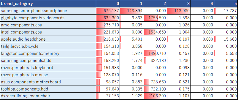
# 各トピックにおける、商品の平均購入数を抽出
display(df_id_cluster2.groupby(['topic']).mean().T)
(EXCELで体裁を整えた↓)

クラスタ0はAsusのPC、1はiPhone、2はLenovoのPCの購入金額が高い、などがわかる。
user_idごとにクラスタ番号をつけてあげる。
# df_martに対してトピック番号をつけてあげる
df_topic_result=df_mart.copy()
top_price_brand_before=df_mart.iloc[:,1:].idxmax(axis=1).values
# user_idごとの所属確率が最も高いトピックを列として追加
df_topic_result['topic_before']=create_topic_no(df_mart, df_data, lda)['topic'].values
# user_idごとの購入額が最も高いブランドを列として追加
df_topic_result['top_price_brand_before']=top_price_brand_before

# df_mart2に対してトピック番号をつけてあげる
df_topic_result2=df_mart2.copy()
top_price_brand_after=df_mart2.iloc[:,1:].idxmax(axis=1).values
# user_idごとの所属確率が最も高いトピックを列として追加
df_topic_result2['topic_after']=create_topic_no(df_mart2, df_data2, lda)['topic'].values
# user_idごとの購入額が最も高いブランドを列として追加
df_topic_result2['top_price_brand_after']=top_price_brand_after

# df_martとdf_mart2をJOIN
df_topic_result=pd.merge(df_topic_result, df_topic_result2[['user_id','topic_after','top_price_brand_after']], on=['user_id'], how='left')
display(df_topic_result)

クラスタのチャートを確認。
# plot Cluster Chart
def pct_abs(pct, raw_data):
absolute = int(np.sum(raw_data)*(pct/100.))
return '{:d}\n({:.0f}%)'.format(absolute, pct) if pct > 5 else ''
def plot_chart(y_km):
km_label=pd.DataFrame(y_km).rename(columns={0:'cluster'})
km_label['val']=1
km_label=km_label.groupby('cluster')[['val']].count().reset_index()
fig=plt.figure(figsize=(5,5))
ax=plt.subplot(1,1,1)
ax.pie(km_label['val'],labels=km_label['cluster'], autopct=lambda p: pct_abs(p, km_label['val']))#, autopct="%1.1f%%")
ax.axis('equal')
ax.set_title('Cluster Chart (ALL UU:{})'.format(km_label['val'].sum()),fontsize=14)
plt.show()
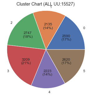
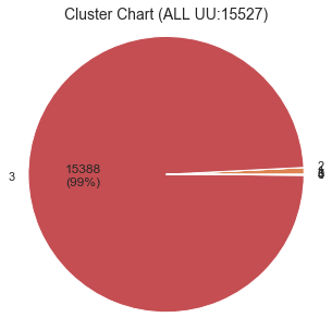
plot_chart(df_topic_result['topic_before'].values)
plot_chart(df_topic_result['topic_after'].values)
前半のデータのチャート
後半のデータのチャート

クラスタごとに特徴が異なるし、クラスタのユーザー数比率も偏っていないので、いい感じに分かれてるような気がする。
クラスタの遷移を確認
前半と後半でクラスタが遷移しているユーザーもいるので、クラスタの遷移をクロス表で見てみる。
display(df_topic_result.pivot_table(index='topic_before', columns='topic_after', values='user_id', aggfunc='count'))
(EXCELで体裁を整えた↓)

例えば、クラスタ2→0への遷移や4→0へ遷移する人が多かったりする。
2→0への遷移した人たちはどういったブランドの購入が増減したのだろうか。ちょっと確認してみる。
購入回数で集計したデータフレームを作成する。
row='user_id'
col='brand_category'
val='order_id'

df_mart=df_pivot(df_before, row, col, val, 'count')
df_mart2=df_pivot(df_after, row, col, val, 'count')

# df_martとdf_mart2で重複していないカラム名をとってくる
after=np.hstack((df_mart.columns.values, df_mart2.columns.values))
unique_after, counts_after = np.unique(after, return_counts=True)
non_dep_after=unique_after[counts_after == 1]

# さっきの重複していないカラム名の中で、df_martに入っていてdf_mart2に入っていないカラム名を抽出
before=np.hstack((non_dep_after, df_mart.columns.values))
unique_before, counts_before = np.unique(before, return_counts=True)
dep_before=unique_before[counts_before != 1]

# df_mart2にdf_mart固有のカラム名の列を追加
for col in dep_before:
    df_mart2[col]=0

# これでdf_martとdf_mart2のカラムがそろう
df_mart=df_mart[df_mart.columns]
df_mart2=df_mart2[df_mart.columns]

display(df_mart)
display(df_mart2)
クラスタ2→0へ遷移した人を抽出。
n=2
m=0
user_id_n_m=df_topic_result[(df_topic_result['topic_before']==n)&(df_topic_result['topic_after']==m)]['user_id'].values
df_b_n_m=df_mart[df_mart['user_id'].isin(user_id_n_m)]
df_a_n_m=df_mart2[df_mart2['user_id'].isin(user_id_n_m)]
display(df_b_n_m)
display(df_a_n_m)

後半のデータから前半のデータを引いて、ブランドごとの購入回数の増減を確認してみる。
df_diff_n_m=df_a_n_m.iloc[:,1:]-df_b_n_m.iloc[:,1:]
df_diff_n_m.index=df_a_n_m['user_id'].values
df_diff_n_m=df_diff_n_m.T
df_diff_n_m['col']=df_diff_n_m.index
df_diff_n_m['brand']=df_diff_n_m['col'].str.split('.', expand=True).iloc[:,0].values
df_diff_n_m=pd.DataFrame(df_diff_n_m.groupby(['brand']).sum().T.sum()).sort_values(0, ascending=False)

# 各ブランドごとの購入回数の増減をプロット
fig=plt.figure(figsize=(20,10))
plt.bar(df_diff_n_m.index[:11], df_diff_n_m[0][:11])
plt.bar(df_diff_n_m.index[-10:], df_diff_n_m[0][-10:])
plt.rcParams["font.family"] = "IPAexGothic"
plt.tick_params(labelsize=18)
plt.xticks(rotation=45)
plt.xlabel('# brand', fontsize=18)
plt.ylabel('# frequency of purchasing', fontsize=18)
plt.title('各ブランドごとの購入回数の増減(上位下位10個ずつ)', fontsize=18)
plt.show()
クラスタ2→0遷移ユーザーのブランド別購入回数の増減
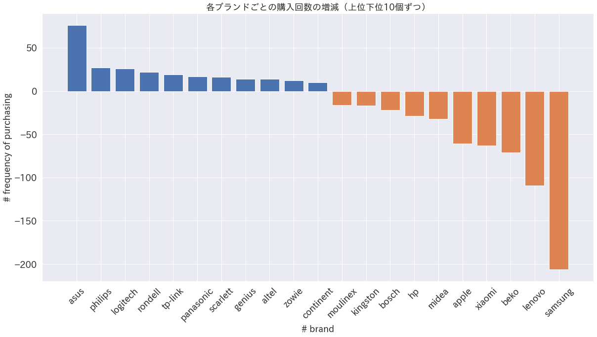
クラスタ2→0に遷移したユーザー群はLENOVOやSamsungの購入回数が減って、AsusやLogitechの購入回数が増えていることがわかる。これは前記のようにクラスタ別の出現確率上位などで確認したクラスタごとの特徴に沿っている。
このように時系列にユーザーの好みの変化を追ったりもできる可能性がある。
また、さらに細かく見ていかないと断定できないが、例えばユーザーのブランドスイッチングが起きてしまった可能性もあったりするので、深堀することで自社や他社のブランドがなぜ売れたか売れなかったの原因を分析していくことができるかもしれない。
以上のようにLDAでクラスタリングすることで意味のある分析ができる可能性がある。
kmeansでクラスタリング
LDAでやったようなクラスタリングをkmeansでもやってみる。
結果のチャートを確認。
row='user_id'
col='brand_category'
val='price'

df_mart=df_pivot(df_before, row, col, val, 'sum')
df_mart2=df_pivot(df_after, row, col, val, 'sum')

# df_martとdf_mart2で重複していないカラム名をとってくる
after=np.hstack((df_mart.columns.values, df_mart2.columns.values))
unique_after, counts_after = np.unique(after, return_counts=True)
non_dep_after=unique_after[counts_after == 1]

# さっきの重複していないカラム名の中で、df_martに入っていてdf_mart2に入っていないカラム名を抽出
before=np.hstack((non_dep_after, df_mart.columns.values))
unique_before, counts_before = np.unique(before, return_counts=True)
dep_before=unique_before[counts_before != 1]

# df_mart2にdf_mart固有のカラム名の列を追加
for col in dep_before:
    df_mart2[col]=0

# これでdf_martとdf_mart2のカラムがそろう
df_mart=df_mart[df_mart.columns]
df_mart2=df_mart2[df_mart.columns]
# LDAに食わせる用の加工
ss=StandardScaler()
df_data=ss.fit_transform(df_mart.iloc[:,1:].values)
ss=StandardScaler()
df_data2=ss.fit_transform(df_mart2.iloc[:,1:].values)

def km_cluster(X, k):
    km=KMeans(n_clusters=k,\
              init="k-means++",\
              random_state=0)
    y_km=km.fit_predict(X)
    return y_km,km

# k=6でクラスタリング
y_km,km=km_cluster(df_data, 6)
plot_chart(y_km)
かなり偏ってクラスタリングされてしまった。
クラスタごとの平均値を見ても多くのクラスタでSamsungが高かったり偏っている。
df_kmeans=df_mart.copy()
df_kmeans['cluster']=y_km
# 各トピックにおける、商品の平均購入数を抽出
df_kmeans.groupby(['cluster']).mean().T
(EXCELで体裁を整えた↓)
以上のように、高次元なデータになるとやはりkmeansではうまくクラスタリングできなかった。
おわりに
POSデータをLDAでクラスタリングしてみた。
距離を指標にクラスタリングするのが難しそうなときに、トピックモデルを使うと良い結果が出るかもしれない。
以上!