はじめに
EMアルゴリズムに出てくるKLダイバージェンスがよくわからなかったので、正規分布間のKLダイバージェンスを求めることでイメージを掴みたいと思います。
KLダイバージェンス
Kullback-Leibler divergence ( KLダイバージェンス、KL情報量 )は、2つの確率分布がどの程度似ているかを表す尺度です。
定義は以下になります。
KL(p||q) = \int_{-\infty}^{\infty}p(x)\ln \frac{p(x)}{q(x)}dx
重要な特性が2点あります。
1つ目は、同じ確率分布では0となるということです。
KL(p||p) = \int_{-\infty}^{\infty}p(x)\ln \frac{p(x)}{p(x)}dx
         = \int_{-\infty}^{\infty}p(x)\ln(1)dx
         = 0
2つ目は、常に0を含む正の値となり、確率分布が似ていない程、大きな値となるということです
これらの特性について正規分布の実例を用いて見ていきます。
正規分布
正規分布の確率密度関数p(x)とq(x)を下記のように定義します。
p(x) = N(\mu_1,\sigma_1^2) = \frac{1}{\sqrt{2\pi\sigma_1^2}} \exp\left(-\frac{(x-\mu_1)^2}{2\sigma_1^2}\right) \\
q(x) = N(\mu_2,\sigma_2^2) = \frac{1}{\sqrt{2\pi\sigma_2^2}} \exp\left(-\frac{(x-\mu_2)^2}{2\sigma_2^2}\right)
正規分布間のKLダイバージェンス
上記2つの正規分布間のKLダイバージェンスを求めます。計算は省略します。
\begin{eqnarray}

KL(p||q)&=& \int_{-\infty}^{\infty}p(x)\ln \frac{p(x)}{q(x)}dx \\
        &=& \cdots \\
        &=& \ln\left(\frac{\sigma_2}{\sigma_1}\right) + \frac{\sigma_1^2+(\mu_1-\mu_2)^2}{2\sigma_2^2} - \frac{1}{2}
\end{eqnarray}
変数が4つもあると分かりにくいので、$p(x)$を平均0、分散1の標準正規分布$N(0,1)$とします。
p(x) =N(0,1)= \frac{1}{\sqrt{2\pi}} \exp\left(-\frac{x^2}{2}\right)
平均が変数のとき
まずは、$q(x)$の標準偏差$\sigma_2$を1として、平均$\mu_2$のみを変数とします。
q(x) =N(\mu_2,1)= \frac{1}{\sqrt{2\pi}} \exp\left(-\frac{(x-\mu_2)^2}{2}\right)
この時のKLダイバージェンスは、
\begin{eqnarray}

KL(p||q) &=& \ln\left(\frac{\sigma_2}{\sigma_1}\right) + \frac{\sigma_1^2+(\mu_1-\mu_2)^2}{2\sigma_2^2} - \frac{1}{2} \\
         &=& \ln\left(\frac{1}{1}\right) + \frac{1^2+(\mu_1-0)^2}{2*1^2} - \frac{1}{2} \\
         &=& \frac{\mu_2^2}{2}
\end{eqnarray}
となります。
$\mu_2$の値を-4から4まで1ずつ増加させた時の、確率分布$q(x)$とKLダイバージェンス$KL(p||q)$の値は以下のようになります。
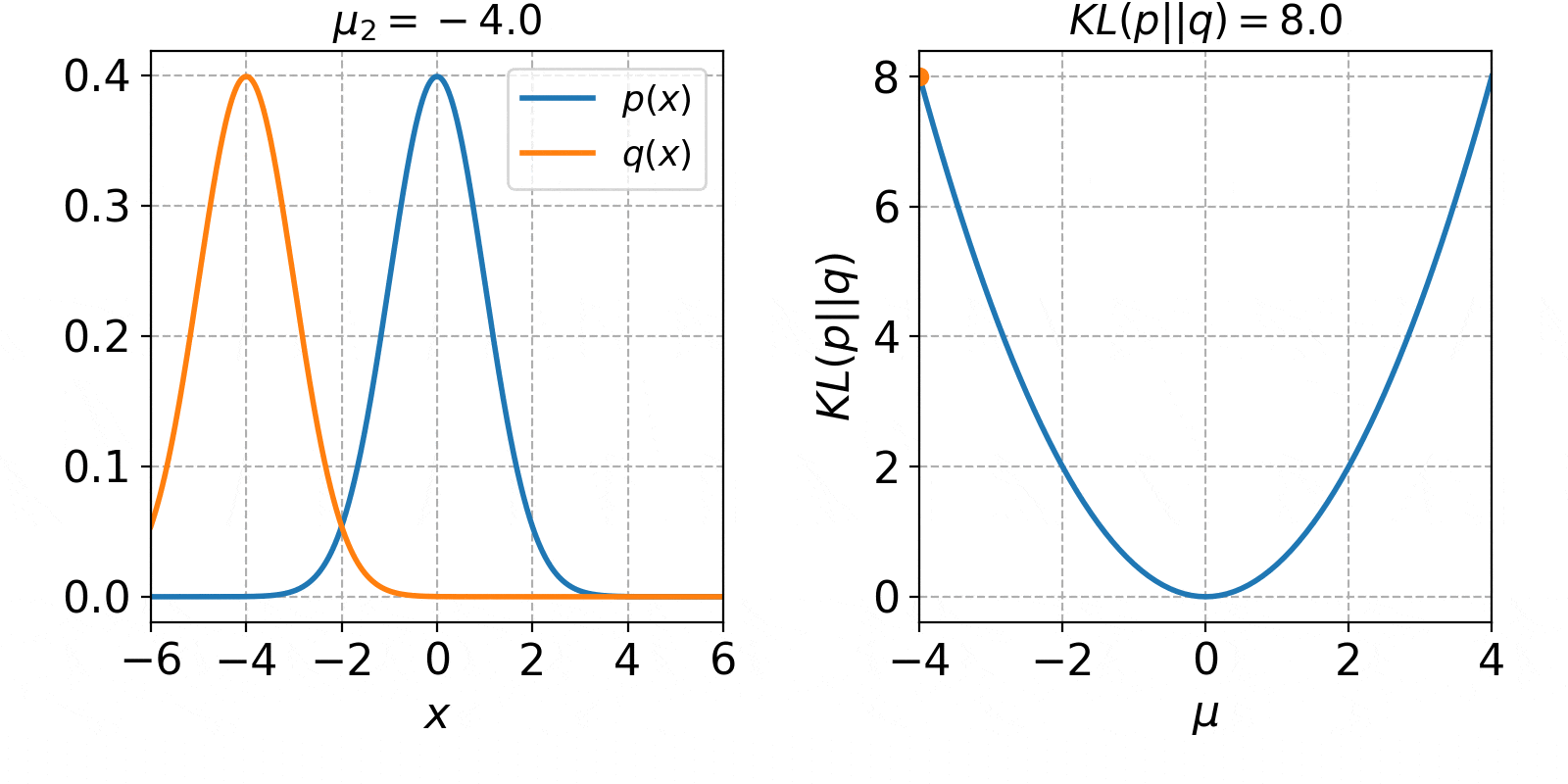
左側のオレンジ色の線が、平均$\mu_2$を変化させた時の$q(x)$です。右側の図は、平均$\mu_2$をx軸に取った時の図になります。青色の線が解析解で、オレンジ色の点が今のKLダイバージェンスの値になります。KLダイバージェンスは、$p(x)$と$q(x)$が完全に一致した時に0となり、離れる程増加していくことが確認できました。
import numpy as np
import matplotlib.pyplot as plt
import matplotlib.animation as animation

# 正規分布
def gaussian1d(x,μ,σ):
    y = 1 / ( np.sqrt(2*np.pi* σ**2 ) )  * np.exp( - ( x - μ )**2  / ( 2 * σ ** 2 ) )
    return y

# 正規分布のKL divergence
def gaussian1d_KLdivergence(μ1,σ1,μ2,σ2):
    A = np.log(σ2/σ1)
    B = ( σ1**2 + (μ1 - μ2)**2 ) / (2*σ2**2)
    C = -1/2
    y = A + B + C
    return y

# KL divergence
def KLdivergence(p,q,dx):
    KL=np.sum(p * np.log(p/q)) * dx
    return KL

# xの刻み
dx  = 0.01

# xの範囲
xlm = [-6,6]

# x座標
x   = np.arange(xlm[0],xlm[1]+dx,dx)

# xの数
x_n   = len(x)

# Case 1
# p(x) = N(0,1)
# q(x) = N(μ,1)

# p(x)の平均μ1
μ1   = 0
# p(x)の標準偏差σ1
σ1   = 1

# p(x)
px   = gaussian1d(x,μ1,σ1)

# q(x)の標準偏差σ2
σ2   = 1

# q(x)の平均μ2
U2   = np.arange(-4,5,1)

U2_n = len(U2)

# q(x)
Qx   = np.zeros([x_n,U2_n])

# KLダイバージェンス
KL_U2  = np.zeros(U2_n)

for i,μ2 in enumerate(U2):
    qx        = gaussian1d(x,μ2,σ2)
    Qx[:,i]   = qx
    KL_U2[i]  = KLdivergence(px,qx,dx)


# 解析解の範囲
U2_exc    = np.arange(-4,4.1,0.1)

# 解析解
KL_U2_exc = gaussian1d_KLdivergence(μ1,σ1,U2_exc,σ2)

# 解析解2
KL_U2_exc2 = U2_exc**2 / 2

#
# plot
#

# figure
fig = plt.figure(figsize=(8,4))
# デフォルトの色
clr=plt.rcParams['axes.prop_cycle'].by_key()['color']

# axis 1
# -----------------------
# 正規分布のプロット
ax = plt.subplot(1,2,1)
# p(x)
plt.plot(x,px,label='$p(x)$')
# q(x)
line,=plt.plot(x,Qx[:,i],color=clr[1],label='$q(x)$')
# 凡例
plt.legend(loc=1,prop={'size': 13})

plt.xticks(np.arange(xlm[0],xlm[1]+1,2))
plt.xlabel('$x$')

# axis 2
# -----------------------
# KLダイバージェンス
ax2 = plt.subplot(1,2,2)
# 解析解
plt.plot(U2_exc,KL_U2_exc,label='Analytical')
# 計算
point, = ax2.plot([],'o',label='Numerical')

# 凡例
# plt.legend(loc=1,prop={'size': 15})

plt.xlim([U2[0],U2[-1]])
plt.xlabel('$\mu$')
plt.ylabel('$KL(p||q)$')

plt.tight_layout()

# 軸に共通の設定
for a in [ax,ax2]:
    plt.axes(a)
    plt.grid()
    # 正方形に
    plt.gca().set_aspect(1/plt.gca().get_data_ratio())

# 更新
def update(i):
    # 線
    line.set_data(x,Qx[:,i])
    # 点
    point.set_data(U2[i],KL_U2[i])

    # タイトル
    ax.set_title("$\mu_2=%.1f$" % U2[i],fontsize=15)
    ax2.set_title('$KL(p||q)=%.1f$' % KL_U2[i],fontsize=15)

# アニメーション
ani = animation.FuncAnimation(fig, update, interval=1000,frames=U2_n)
# plt.show()
# ani.save("KL_μ.gif", writer="imagemagick")
標準偏差が変数のとき
続いて$q(x)$の平均$\mu_2$を0として、標準偏差$\sigma_2$のみを変数とします。
q(x) =N(0,\sigma^2_2)= \frac{1}{\sqrt{2\pi\sigma_2^2}} \exp\left(-\frac{x^2}{2\sigma_2^2}\right)
この時のKLダイバージェンスは、
\begin{eqnarray}

KL(p||q) &=& \ln\left(\frac{\sigma_2}{\sigma_1}\right) + \frac{\sigma_1^2+(\mu_1-\mu_2)^2}{2\sigma_2^2} - \frac{1}{2} \\
         &=& \ln\left(\frac{\sigma_2}{1}\right) + \frac{1^2}{2\sigma_2^2} - \frac{1}{2} \\
         &=& \ln\left(\sigma_2\right) + \frac{1}{2\sigma_2^2} - \frac{1}{2} \\
\end{eqnarray}
となります。
$\sigma_2$の値を0.5から4まで変化させた時の、確率分布$q(x)$とKLダイバージェンス$KL(p||q)$の値は以下のようになります。
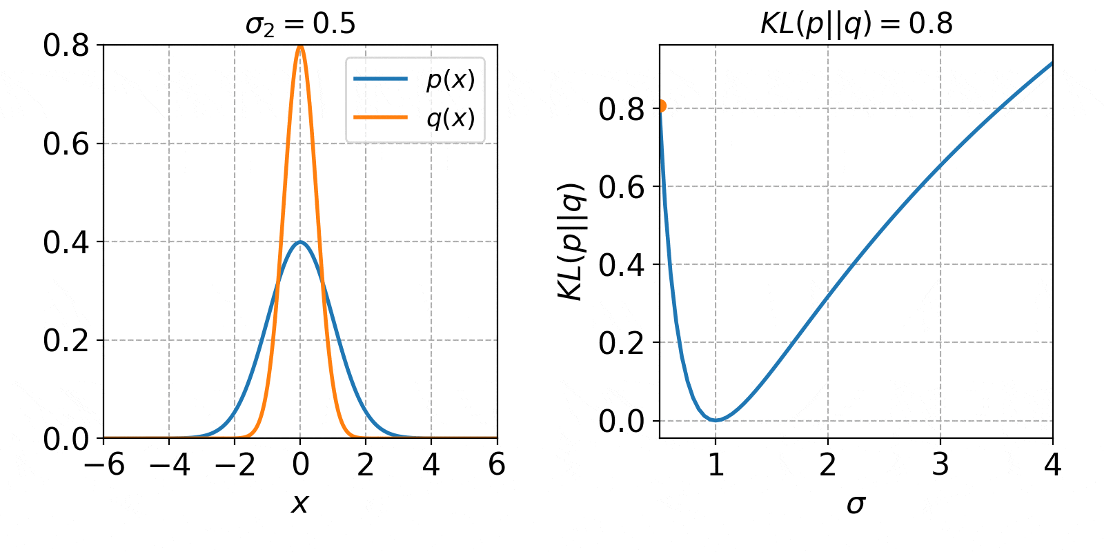
KLダイバージェンスの変化は、先程と同じく確率分布が一致した時に0となり、形状が異なる程増加していくという特徴が見られました。
import numpy as np
import matplotlib.pyplot as plt
import matplotlib.animation as animation

# 正規分布
def gaussian1d(x,μ,σ):
    y = 1 / ( np.sqrt(2*np.pi* σ**2 ) )  * np.exp( - ( x - μ )**2  / ( 2 * σ ** 2 ) )
    return y

# 正規分布のKL divergence
def gaussian1d_KLdivergence(μ1,σ1,μ2,σ2):
    A = np.log(σ2/σ1)
    B = ( σ1**2 + (μ1 - μ2)**2 ) / (2*σ2**2)
    C = -1/2
    y = A + B + C
    return y

# KL divergence
def KLdivergence(p,q,dx):
    KL=np.sum(p * np.log(p/q)) * dx
    return KL

# xの刻み
dx  = 0.01

# xの範囲
xlm = [-6,6]

# x座標
x   = np.arange(xlm[0],xlm[1]+dx,dx)

# xの数
x_n   = len(x)

# Case 2
# p(x) = N(0,1)
# q(x) = N(0,σ**2)

# p(x)の平均μ1
μ1   = 0
# p(x)の標準偏差σ1
σ1   = 1

# p(x)
px   = gaussian1d(x,μ1,σ1)

# q(x)の平均μ2
μ2   = 0

# q(x)の標準偏差σ2
S2   = np.hstack([ np.arange(0.5,1,0.1),np.arange(1,2,0.2),np.arange(2,4.5,0.5) ])

S2_n = len(S2)

# q(x)
Qx   = np.zeros([x_n,S2_n])

# KLダイバージェンス
KL_S2  = np.zeros(S2_n)

for i,σ2 in enumerate(S2):
    qx        = gaussian1d(x,μ2,σ2)
    Qx[:,i]   = qx
    KL_S2[i]  = KLdivergence(px,qx,dx)


# 解析解の範囲
S2_exc    = np.arange(0.5,4+0.05,0.05)

# 解析解
KL_S2_exc = gaussian1d_KLdivergence(μ1,σ1,μ2,S2_exc)

# 解析解2
KL_S2_exc2 = np.log(S2_exc) + 1/(2*S2_exc**2) - 1 / 2

#
# plot
#

# figure
fig = plt.figure(figsize=(8,4))
# デフォルトの色
clr=plt.rcParams['axes.prop_cycle'].by_key()['color']

# axis 1
# -----------------------
# 正規分布のプロット
ax = plt.subplot(1,2,1)
# p(x)
plt.plot(x,px,label='$p(x)$')
# q(x)
line,=plt.plot(x,Qx[:,i],color=clr[1],label='$q(x)$')
# 凡例
plt.legend(loc=1,prop={'size': 13})

plt.ylim([0,0.8])
plt.xticks(np.arange(xlm[0],xlm[1]+1,2))
plt.xlabel('$x$')

# axis 2
# -----------------------
# KLダイバージェンス
ax2 = plt.subplot(1,2,2)
# 解析解
plt.plot(S2_exc,KL_S2_exc,label='Analytical')
# 計算
point, = ax2.plot([],'o',label='Numerical')

# 凡例
# plt.legend(loc=1,prop={'size': 15})

plt.xlim([S2[0],S2[-1]])
plt.xlabel('$\sigma$')
plt.ylabel('$KL(p||q)$')

plt.tight_layout()

# 軸に共通の設定
for a in [ax,ax2]:
    plt.axes(a)
    plt.grid()
    # 正方形に
    plt.gca().set_aspect(1/plt.gca().get_data_ratio())

# 更新
def update(i):
    # 線
    line.set_data(x,Qx[:,i])
    # 点
    point.set_data(S2[i],KL_S2[i])

    # タイトル
    ax.set_title("$\sigma_2=%.1f$" % S2[i],fontsize=15)
    ax2.set_title('$KL(p||q)=%.1f$' % KL_S2[i],fontsize=15)

# アニメーション
ani = animation.FuncAnimation(fig, update, interval=1000,frames=S2_n)
plt.show()
# ani.save("KL_σ.gif", writer="imagemagick")
平均、標準偏差が変数のとき
平均$\mu_2$と標準偏差$\sigma_2$の両方を変化させた時の、KLダイバージェンスの値をプロットしたのが下記になります。

import numpy as np
import matplotlib.pyplot as plt

# 正規分布
def gaussian1d(x,μ,σ):
    y = 1 / ( np.sqrt(2*np.pi* σ**2 ) )  * np.exp( - ( x - μ )**2  / ( 2 * σ ** 2 ) )
    return y

# 正規分布のKL divergence
def gaussian1d_KLdivergence(μ1,σ1,μ2,σ2):
    A = np.log(σ2/σ1)
    B = ( σ1**2 + (μ1 - μ2)**2 ) / (2*σ2**2)
    C = -1/2
    y = A + B + C
    return y

# KL divergence
def KLdivergence(p,q,dx):
    KL=np.sum(p * np.log(p/q)) * dx
    return KL

def Motion(event):
    global cx,cy,cxid,cyid

    xp = event.xdata
    yp = event.ydata

    if (xp is not None) and (yp is not None):
        gca = event.inaxes

        if gca is axs[0]:
            cxid,cx = find_nearest(x,xp)
            cyid,cy = find_nearest(y,yp)

            lns[0].set_data(G_x,Qx[:,cxid,cyid])
            lns[1].set_data(x,Z[:,cyid])
            lns[2].set_data(y,Z[cxid,:])


            lnhs[0].set_ydata([cy,cy])
            lnvs[0].set_xdata([cx,cx])

            lnvs[1].set_xdata([cx,cx])
            lnvs[2].set_xdata([cy,cy])


        if gca is axs[2]:
            cxid,cx = find_nearest(x,xp)

            lns[0].set_data(G_x,Qx[:,cxid,cyid])
            lns[2].set_data(y,Z[cxid,:])
            lnvs[0].set_xdata([cx,cx])
            lnvs[1].set_xdata([cx,cx])

        if gca is axs[3]:
            cyid,cy = find_nearest(y,xp)

            lns[0].set_data(G_x,Qx[:,cxid,cyid])
            lns[1].set_data(x,Z[:,cyid])
            lnhs[0].set_ydata([cy,cy])
            lnvs[2].set_xdata([cy,cy])

    axs[1].set_title("$\mu_2=%5.2f, \sigma_2=$%5.2f" % (cx,cy),fontsize=15)
    axs[0].set_title('$KL(p||q)=$%.3f' % Z[cxid,cyid],fontsize=15)

    plt.draw()

def find_nearest(array, values):
    id = np.abs(array-values).argmin()
    return id,array[id]

# xの刻み
G_dx  = 0.01
# xの範囲
G_xlm = [-4,4]
# x座標
G_x   = np.arange(G_xlm[0],G_xlm[1]+G_dx,G_dx)
# xの数
G_n   = len(G_x)

# p(x)の平均μ1
μ1   = 0
# p(x)の標準偏差σ1
σ1   = 1
# p(x)
px   = gaussian1d(G_x,μ1,σ1)

# q(x)の平均μ2
μ_lim = [-2,2]
μ_dx  = 0.1
μ_x   = np.arange(μ_lim[0],μ_lim[1]+μ_dx,μ_dx)
μ_n   = len(μ_x)

# q(x)の標準偏差σ2
σ_lim = [0.5,4]
σ_dx  = 0.05
σ_x   = np.arange(σ_lim[0],σ_lim[1]+σ_dx,σ_dx)
σ_n   = len(σ_x)

# KLダイバージェンス
KL   = np.zeros([μ_n,σ_n])
# q(x)
Qx   = np.zeros([G_n,μ_n,σ_n])

for i,μ2 in enumerate(μ_x):
    for j,σ2 in enumerate(σ_x):
        KL[i,j]   = gaussian1d_KLdivergence(μ1,σ1,μ2,σ2)
        Qx[:,i,j] = gaussian1d(G_x,μ2,σ2)

x   = μ_x
y   = σ_x

X,Y = np.meshgrid(x,y)
Z   = KL

cxid  = 0
cyid  = 0

cx    = x[cxid]
cy    = y[cyid]

xlm   = [ x[0], x[-1] ]
ylm   = [ y[0], y[-1] ]

axs   = []
ims   = []
lns   = []
lnvs  = []
lnhs  = []

# figure
# ----------------
plt.close('all')
plt.figure(figsize=(8,8))
# デフォルトの色
clr=plt.rcParams['axes.prop_cycle'].by_key()['color']

# フォントサイズ
plt.rcParams["font.size"] = 16
# 線幅
plt.rcParams['lines.linewidth'] = 2
# gridのlinestyleを点線に
plt.rcParams["grid.linestyle"] = '--'

# plot時の範囲のマージンをなくす
plt.rcParams['axes.xmargin'] = 0.

# ax1
# ----------------
ax = plt.subplot(2,2,1)

Interval = np.arange(0,8,0.1)
plt.plot(μ1,σ1,'rx',label='$(μ_1,σ_1)=(0,1)$')
im = plt.contourf(X,Y,Z.T,Interval,cmap='hot')
lnv= plt.axvline(x=cx,color='w',linestyle='--',linewidth=1)
lnh= plt.axhline(y=cy,color='w',linestyle='--',linewidth=1)

ax.set_title('$KL(p||q)=$%.3f' % Z[cxid,cyid],fontsize=15)
plt.xlabel('μ')
plt.ylabel('σ')

axs.append(ax)
lnhs.append(lnh)
lnvs.append(lnv)
ims.append(im)

# ax2
# ----------------
ax = plt.subplot(2,2,2)
plt.plot(G_x,px,label='$p(x)$')
ln, = plt.plot(G_x,Qx[:,cxid,cyid],color=clr[1],label='$q(x)$')
plt.legend(prop={'size': 10})
ax.set_title("$\mu_2=%5.2f, \sigma_2=$%5.2f" % (cx,cy),fontsize=15)

axs.append(ax)
lns.append(ln)
plt.grid()

# ax3
# ----------------
ax = plt.subplot(2,2,3)
ln,=plt.plot(x,Z[:,cyid])
lnv= plt.axvline(x=cx,color='k',linestyle='--',linewidth=1)

plt.ylim([0,np.max(Z)])
plt.grid()
plt.xlabel('μ')
plt.ylabel('KL(p||q)')

lnvs.append(lnv)
axs.append(ax)
lns.append(ln)

# ax4
# ----------------
ax = plt.subplot(2,2,4)
ln,=plt.plot(y,Z[cxid,:])

lnv= plt.axvline(x=cy,color='k',linestyle='--',linewidth=1)

plt.ylim([0,np.max(Z)])
plt.xlim([ylm[0],ylm[1]])
plt.grid()

plt.xlabel('σ')
plt.ylabel('KL(p||q)')

lnvs.append(lnv)
axs.append(ax)
lns.append(ln)

plt.tight_layout()

for ax in axs:
    plt.axes(ax)
    ax.set_aspect(1/ax.get_data_ratio())

plt.connect('motion_notify_event', Motion)

plt.show()