高速道路の設計(クロソイド曲線)
S字の道路をシミュレータ上で作ったら、緩和区間ないといけないと指摘された。
調べてみて、緩和区間は下記がわかりやすいと思う。
【測量士】緩和曲線(クロソイド)の基礎知識②:曲率とクロソイド基本式
で、緩和区間の長さは法規で決まってる。
緩和区間の法規(P.7,8)
よし、これで作れると思ったら、シミュレータ上での指定方法が、
円弧半径の開始、終了と角度になってる。orz。長さいくつ?
なので、本腰入れて調べてみた。
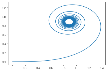
まずクロソイド曲線を描いてみる
よくある絵。こんなに渦まかなくてもよかったかも。。。
import numpy as np
from scipy import integrate
import matplotlib.pyplot as plt

t = np.arange(0, 16, 0.01)
x = np.cos(t**2 / 2)
y = np.sin(t**2 / 2)

x_int = integrate.cumtrapz(x, t, initial=0)
y_int = integrate.cumtrapz(y, t, initial=0)

plt.plot(x_int, y_int)
plt.show()
円弧半径と角度の関係を調べる
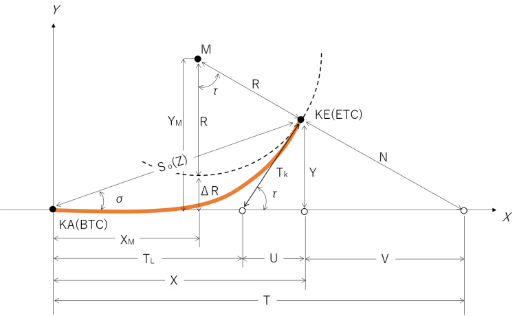
図はここから引用。
やりたいことは、R+ΔR, R, τ が与えられたときにオレンジ色の線の長さを知りたい。
ここ にドンピシャなものがあった。$A$(クロソイドパラメータ)を使って式を直す。
 \tau =\dfrac{k\omega }{2}(\dfrac{L}{v})^2 = \dfrac{L^2}{2 A^2} = \dfrac{L}{2 R} \\
 \because A^2=RL=\dfrac{v^2}{k\omega }
材料はそろったので解いてみる
定義
R_1  = 円弧半径(開始) \\
R_2  = 円弧半径(終了) \\
\tau_2 - \tau_1 = 角度 = \tau \\
L = L_2 - L_1
$L$を求めたい
計算
A^2 = R_1 L_1 = R_2 L_2 \\
L_1 = 2 R_1 \tau_1 \\
L_2 = 2 R_2 \tau_2 \\

\therefore \tau_2 = (\dfrac{R_1}{R_2})^2 \tau_1
\tau_2 - \tau_1 = ((\dfrac{R_1}{R_2})^2 - 1) \tau_1 = \tau \\
\tau_1 = \dfrac{\tau {R_2}^2}{{R_1}^2 - {R_2}^2} \\
L_1 = \dfrac{2 \tau {R_1} {R_2}^2}{{R_1}^2 - {R_2}^2} \\
L_2 = \dfrac{2 \tau {R_1}^2 {R_2}}{{R_1}^2 - {R_2}^2} \\
\\
L = L_2 - L_1 = \dfrac{2 \tau R_1 R_2}{R_1 + R_2} \\

R_1 \to \infty \verb|の場合| L_1 = 0, L = 2 \tau R_2
書いてみる
import numpy as np
from scipy import integrate
import matplotlib.pyplot as plt

def rotate(rad, x, y):
    rot = np.array([[np.cos(rad), -np.sin(rad)],
                    [np.sin(rad), np.cos(rad)]])
    tmp = np.dot(rot, np.array([x, y]))
    return tmp[0], tmp[1]

# X= A √2τ(1 - tau^2/(2!*5) + ... + (-tau^2)^n / (2n! * (4n+1)))
# Pk = Pk-1×(-1)/((2k-2)×(2k-3))×τ^2
# Qk = Pk/(4k-3)
def calc_clothoid_x(A, tau, Er=0.001):
    b = A * np.sqrt(2 * tau) #  共通項
    s = 1 # カッコ内合計
    k = 1 # 第k項のk
    pk = 1 # X: (-1)/((2k-2)×(2k-3))×τ^2
    last = 0
    x = b * s
    while np.abs(x - last) >= Er:
        last = x # 前回の値を保存
        k += 1
        pk = pk * (-1) / ((2*k-2) * (2*k-3)) * tau * tau
        qk = pk / (4*k - 3)
        s += qk
        x = b * s
    return x

# Y = Aτ√2τ(1/3 - tau^2/(3!*7) + ... + (-tau^2)^n / ((2n+1)! + (4n+3)))
# Pk = Pk-1×(-1)/((2k-1)×(2k-2))×τ^2
# Qk = Pk/(4k-1)
def calc_clothoid_y(A, tau, Er=0.001):
    b = A * tau * np.sqrt(2 * tau) #  共通項
    s = 1 / 3 # カッコ内合計
    k = 1 # 第k項のk
    pk = 1 # X: (-1)/((2k-2)×(2k-3))×τ^2
    last = 0
    y = b * s
    while np.abs(y - last) >= Er:
        last = y # 前回の値を保存
        k += 1
        pk = pk * (-1) / ((2*k-1) * (2*k-2)) * tau * tau
        qk = pk / (4*k - 1)
        s += qk
        y = b * s
    return y

def plot_clothoid1(R1, R2, tau, v=0):
    tau1 = np.deg2rad(tau) / ((R1/R2)**2 - 1)
    tau2 = tau1 * ((R1/R2)**2)

    L1 = 2 * R1 * tau1
    L2 = 2 * R2 * tau2
    L = L2 - L1
    A2 = np.abs(R2*L2) # R1 < R2 に備えて
    A = np.sqrt(A2)

    l = np.linspace(L1, L2, int(L / 0.01))
    x = np.cos(l**2 / (2 * A2))
    y = np.sin(l**2 / (2 * A2))

    x_int = integrate.cumtrapz(x, l, initial=0)
    y_int = integrate.cumtrapz(y, l, initial=0)

    X2 = x_int[-1]
    Y2 = y_int[-1]
    sigma = np.arctan2(Y2, X2)
    X2m = X2 - R2 * np.sin(tau2)
    Y2m = Y2 + R2 * np.cos(tau2)
    d_R2 = Y2m - R2

    tk = Y2 / np.sin(tau2)
    tl = X2 - Y2 / np.tan(tau2)
    so = Y2 / np.sin(sigma)


    print("(R1, R2, tau) = (%.1f, %.1f, %.1f(%.4f))" % (R1, R2, tau, np.deg2rad(tau)))
    print("(tau1, tau2) = (%.1f, %.1f)" % (np.rad2deg(tau1), np.rad2deg(tau2)))
    print("A = %.1f" % A)
    print("L = %.1f" % L)
    if v > 0:
        # v[km/h]
        print("(V, P) = (%d, %.3f)" % (v, ((v/3.6)**3) / np.abs(R2*L2) ))

    print("(X, Y, σ)@L2 = (%.4f, %.4f, %.4f)" % (X2, Y2, sigma))
    print("(Xm, Ym, ΔR)@L2 = (%.4f, %.4f, %.4f)" % (X2m, Y2m, d_R2))
    print("(Tk, Tl, So)@L2 = (%.4f, %.4f, %.4f)" % (tk, tl, so))
    if tau2 > 0:
        #print(x_int[-1], y_int[-1])
        print(calc_clothoid_x(A, tau2), calc_clothoid_y(A, tau2))


    plt.axes().set_aspect('equal')
    plt.plot(x_int, y_int)
    plt.show()

    rot = -np.arctan2(y[0], x[0])
    if not np.isclose(0, rot, atol=0.01):
        print("rot=", np.rad2deg(rot))
        x_rot, y_rot = rotate(rot, x_int, y_int)

        plt.axes().set_aspect('equal')
        plt.plot(x_rot, y_rot)
        plt.show()

def plot_clothoid2(R, L, R0 = 100000, v=0):
    tau = L * (R + R0) / 2 / R / R0
    plot_clothoid1(R0, R, np.rad2deg(tau), v=v)

def plot_clothoid3(R, A, R0 = 100000, v=0):
    tau = A*A * (R*R + R0*R0) / 2 / R / R / R0 / R0
    plot_clothoid1(R0, R, np.rad2deg(tau), v=v)

def plot_clothoid4(R, v, R0 = 100000, t=3):
    tau = v / 3.6 * t * (R + R0) / 2 / R / R0
    plot_clothoid1(R0, R, np.rad2deg(tau), v=v)


plot_clothoid3(R=50, A=40, v=40)

plot_clothoid1(50, 30, 180, v=40)
plot_clothoid1(30, 50, 90, v=40)
plot_clothoid1(100000, 50, 30, v=40)
plot_clothoid2(50, 35, v=40)
# plot_clothoid3(50, 40, v=40)
plot_clothoid3(50, 43, v=40)
# plot_clothoid3(50, 45, v=40)
plot_clothoid4(50, 40)
設計速度:40km/h でR50の場合、クロソイドパラメータを43にすると下記になる。
- 角度:21.2°
- 緩和区間:37m
- 躍度: 0.74(ショーツ式)
注意:τでべき級数展開したものと値が違う。べき級数展開した方は
クロソイドの計算(xls)とも一致したからintegrate.cumtrapzの方が間違っていると思うけど。。。
(R1, R2, tau) = (100000.0, 50.0, 21.2(0.3698))
(tau1, tau2) = (0.0, 21.2)
A = 43.0
L = 37.0
(V, P) = (40, 0.742)
(X, Y, σ)@L2 = (36.4590, 4.5141, 0.1232)
(Xm, Ym, ΔR)@L2 = (18.3876, 51.1341, 1.1341)
(Tk, Tl, So)@L2 = (12.4895, 24.8138, 36.7374)
36.477500292592346 4.5140730696816025
緩和区間を省略できるケースもあるみたいだけど、今回のシミュレーションでは関係なさそうなので無視。
本当は、片勾配や道幅も考慮する必要があるけど、無視していいかな。。。
参考
- 高速道路の設計(クロソイド曲線) 数学的には一番わかりやすい。けど東大受験生すげーな、解説は理解できても問題解くのは無理。
- 千三つさんが教える土木工学 - 3.5 平面線形 記号の使い方とかなんか独特感がある。質量m[kg]じゃなくてG[N]は、単位の違いにすぐ気が付かず参った。
- 千三つさんが教える土木工学 - 10.3 緩和曲線
- 【測量士】緩和曲線(クロソイド)の基礎知識②:曲率とクロソイド基本式 ①~④も参考になる
- クロソイドの設計と作図 パラメータと半径の目安 が参考になる
- 【平面線形】クロソイドがある場合の最小曲線長について詳しく解説します
- 緩和区間の法規(P.7,8)
- クロソイド曲線 VBScript
- オガワ設計技術 - ダウンロード