「口コミサイトの点数は,単価が高いと事前の期待値が高い分低くなりやすく,安いと逆に高くなりやすい」
と言っている人がいたので確かめてみました.
逆に,**高いお金を払ったときほど,支出を正当化する認知バイアスが働くのでは?**と思った次第です.
データ
- グルメサイトのスコアと予算
- 都内に限定
- ディナーに限定
- 予算が幅をもつときは最低金額
- 標本の大きさ:10000
結果
Call:
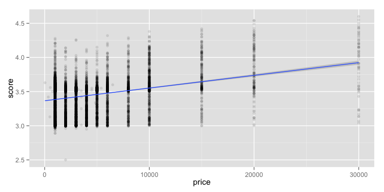
lm(formula = score ~ price, data = src)
Residuals:
Min 1Q Median 3Q Max
-0.90321 -0.19760 0.07802 0.15538 0.89540
Coefficients:
Estimate Std. Error t value Pr(>|t|)
(Intercept) 3.366e+00 3.185e-03 1056.91 <2e-16 ***
price 1.860e-05 5.575e-07 33.35 <2e-16 ***
---
Signif. codes: 0 ‘***’ 0.001 ‘**’ 0.01 ‘*’ 0.05 ‘.’ 0.1 ‘ ’ 1
Residual standard error: 0.2353 on 9998 degrees of freedom
Multiple R-squared: 0.1001, Adjusted R-squared: 0.1
F-statistic: 1112 on 1 and 9998 DF, p-value: < 2.2e-16
やはり単価が高いほどスコアが高くなる傾向があるようです.
一般化線形モデルを使う場合,スコアを0〜1に正規化して,応答変数がベータ分布に従うと仮定するのが良いのでしょうか?
Call:
betareg(formula = score ~ price, data = src)

Standardized weighted residuals 2:
    Min      1Q  Median      3Q     Max
-3.4628 -0.8374  0.2806  0.6340  4.8823

Coefficients (mean model with logit link):
             Estimate Std. Error z value Pr(>|z|)
(Intercept) 7.156e-01  3.010e-03  237.76   <2e-16 ***
price       1.938e-05  5.497e-07   35.25   <2e-16 ***

Phi coefficients (precision model with identity link):
      Estimate Std. Error z value Pr(>|z|)
(phi)   94.290      1.327   71.04   <2e-16 ***
---
Signif. codes:  0 '***' 0.001 '**' 0.01 '*' 0.05 '.' 0.1 ' ' 1

Type of estimator: ML (maximum likelihood)
Log-likelihood: 1.632e+04 on 3 Df
Pseudo R-squared: 0.1228
Number of iterations: 8 (BFGS) + 2 (Fisher scoring)
居酒屋
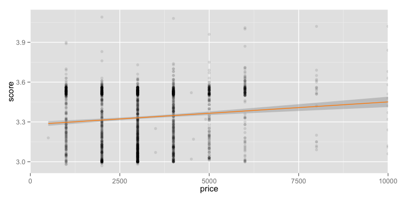
単一のカテゴリの中で比較すると結果が変わってくるかもと思い,対象を居酒屋に限定してみました.
標本の大きさは2000です.
Call:
lm(formula = score ~ price, data = src)

Residuals:
     Min       1Q   Median       3Q      Max
-0.39076 -0.20677  0.03257  0.19190  0.77612

Coefficients:
             Estimate Std. Error t value Pr(>|t|)
(Intercept) 3.280e+00  1.031e-02 318.215  < 2e-16 ***
price       1.711e-05  2.842e-06   6.021 2.05e-09 ***
---
Signif. codes:  0 ‘***’ 0.001 ‘**’ 0.01 ‘*’ 0.05 ‘.’ 0.1 ‘ ’ 1

Residual standard error: 0.2119 on 1998 degrees of freedom
Multiple R-squared:  0.01782,	Adjusted R-squared:  0.01733
F-statistic: 36.25 on 1 and 1998 DF,  p-value: 2.055e-09
同じ傾向でした.