はじめに
気候予測データセット2022の「日本域気候予測データ2㎞版」格子点データをラスタ化する際の投影パラメータを同定しました。
前回に続き、「日本域気候予測データ―格子点データ」2㎞版の投影パラメータを同定します。
「日本域気候予測データ-格子点データ」2㎞版の入手とマップ化の記事はこちら。
モデル格子情報の入手
気候予測データセット(DS2022)から、日本域気候予測データのモデル格子情報を入手します。
ファイルは次の3つ。
- cnst_2km.dat
- cnst_2km.ctl
- cnst_2km.csv
データの入手方法は以下を参考にしてください。
ctlファイルのPDEF情報
cnst_2km.ctl
DSET ^cnst_2km.dat
OPTIONS big_endian
title constant data
undef -999.9
pdef 485 1681 LCCR 44 144 178 1474 30 60 80 2000 2000
xdef  2300 linear 114  0.02
ydef  2000 linear 16   0.02
zdef    1 linear 1 1
tdef 1 linear 00z01SEP1980 1hr
vars   4
FLAT  1 99 deg
FLON  1 99 deg
ZS    1 99 m
SL    1 99 sl
endvars
PDEF行を読み解くと、
pdef情報.
pdef 485 1681 LCCR 44 144 178 1474 30 60 80 2000 2000
↓
isize:485	The size of the native grid in the x direction
jsize:1681	The size of the native grid in the y direction
projection:LCCR the Lambert Conformal projection
latref:44	reference latitude
lonref:144	reference longitude (in degrees, E is positive, W is negative)
iref:178	i of ref point
jref:1474	j of ref point
Struelat:30	S true lat
Ntruelat:60	N true lat
slon:80	standard longitude
dx:2000	grid X increment in meters
dy:2000	grid Y increment in meters
となります。
Projectionの同定
座標系は5㎞版と同じで、PROJ.4文字列にすると、
PROJ.4 String
+proj=lcc +lat_1=30.0 +lat_2=60.0 +lon_0=80. +lat_0=0 +x_0=0 +y_0=0 +a=6371000 +b=6371000 +units=m +no_defs
になります。
GeoTransFormパラメータの同定
ctlファイルのPDEF情報から、
Python
GT(2) = GT(4) = 0
GT(1) = 2000
GT(5) = -2000
になります。
GT(0)とGT(3)については、cnst_2km.csvからupper-left pixelの座標を特定できます。
Python
import os
import pandas as pd

os.chdir("/mnt/c/Users/hoge/JWP9")

# cnst_2km.csvを読み込む
cnst_df = pd.read_csv("./dias/data/jmagwp/gwp9/meta_2km/cnst_2km.csv")
cnst_df.columns = ["x","y","flat","flon","zs","sl"]

# upper-left pixelの座標を特定
ul_lat,ul_lon = cnst_df.loc[(cnst_df["x"]==1)&(cnst_df["y"]==1681),["flat","flon"]].values[0]

print(ul_lat,ul_lon)
# →49.128177642822266 144.71006774902344
ランベルト正角円錐図法の座標系に変換し、右上角の座標を同定します。
Python
from osgeo import gdal, gdalconst, gdal_array
from osgeo import osr

#緯度経度座標系のインスタンスを作成
src_srs = osr.SpatialReference()
src_srs.ImportFromEPSG(4326)

#ランベルト正角円錐図法座標系のインスタンスを作成
outRasterSRS = osr.SpatialReference()
outRasterSRS.ImportFromProj4(
"+proj=lcc +lat_1=30.0 +lat_2=60.0 +lon_0=80. +lat_0=0 +x_0=0 +y_0=0 +a=6371000 +b=6371000 +units=m +no_defs")

#緯度経度をランベルト正角円錐図法の座標系に変換
trans = osr.CoordinateTransformation(src_srs,outRasterSRS)

ul_x,ul_y,Z = trans.TransformPoint(ul_lat,ul_lon)

#ひだり上の角の位置を計算
ul_x = ul_x - 1000
ul_y = ul_y + 1000

print(ul_x,ul_y)
# →4074196.5514666005 7530619.71549598
結果、GeoTransFormのパラメータは
Python
[4074196.5514666005,2000,0,7530619.71549598,0,-2000]
となります。
海陸比データをGeoTIFF化
同定したパラメータの検証のため、海陸比データをGeoTiff化します。
Python
import os
import numpy as np
from osgeo import gdal, gdalconst, gdal_array
from osgeo import osr

os.chdir("/mnt/c/Users/hoge/JWP9")

#モデル格子点情報を読み込む
cnst_dat = np.fromfile("./dias/data/jmagwp/gwp9/meta_2km/cnst_2km.dat",dtype='>f4')
var_arr =  cnst_dat.reshape(4,815285)
sl_arr = var_arr[3].reshape(1681,485)[::-1,:]

#GeoTiFFを作成
name = "cnst_2km_sl.gtiff"
output = gdal.GetDriverByName('GTiff').Create(name,485,1681,1,gdal.GDT_Float64)

#Projectionを設定
outRasterSRS = osr.SpatialReference()
outRasterSRS.ImportFromProj4(
"+proj=lcc +lat_1=30.0 +lat_2=60.0 +lon_0=80. +lat_0=0 +x_0=0 +y_0=0 +a=6371000 +b=6371000 +units=m +no_defs")
output.SetProjection(outRasterSRS.ExportToWkt())

#GeoTransformを設定
output.SetGeoTransform([4074196.5514666005,2000,0,7530619.71549598,0,-2000])

#海陸比データを設定
outband = output.GetRasterBand(1)
outband.WriteArray(sl_arr.astype("float64"))

outband.FlushCache()
output =None
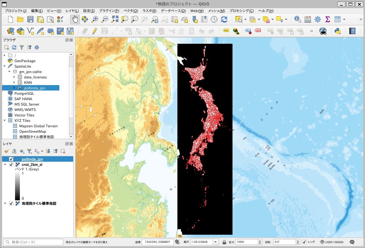
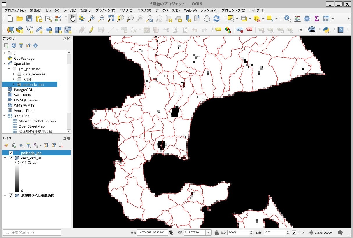
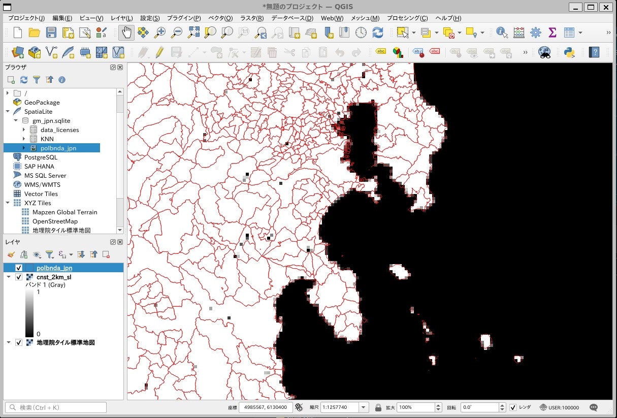
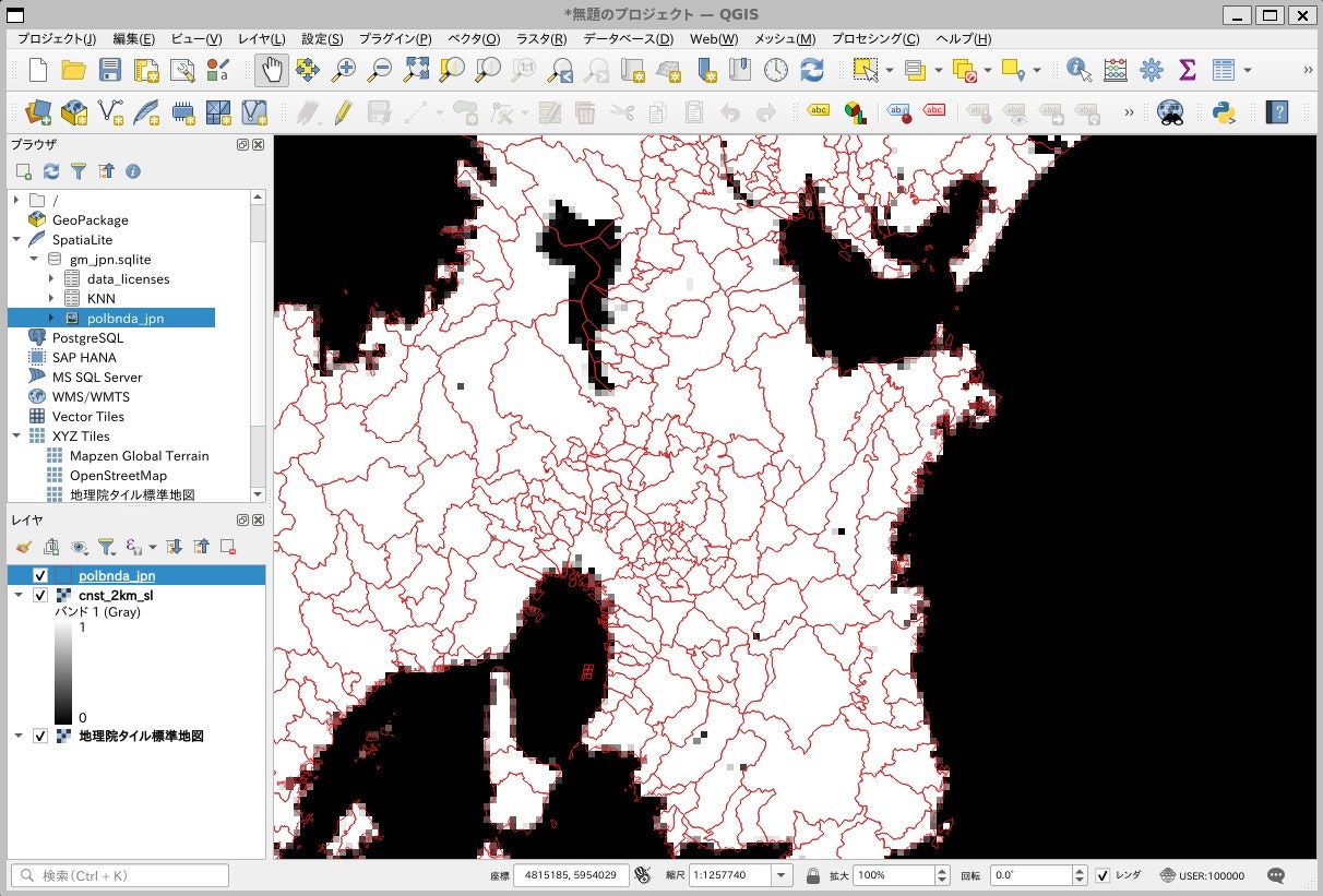
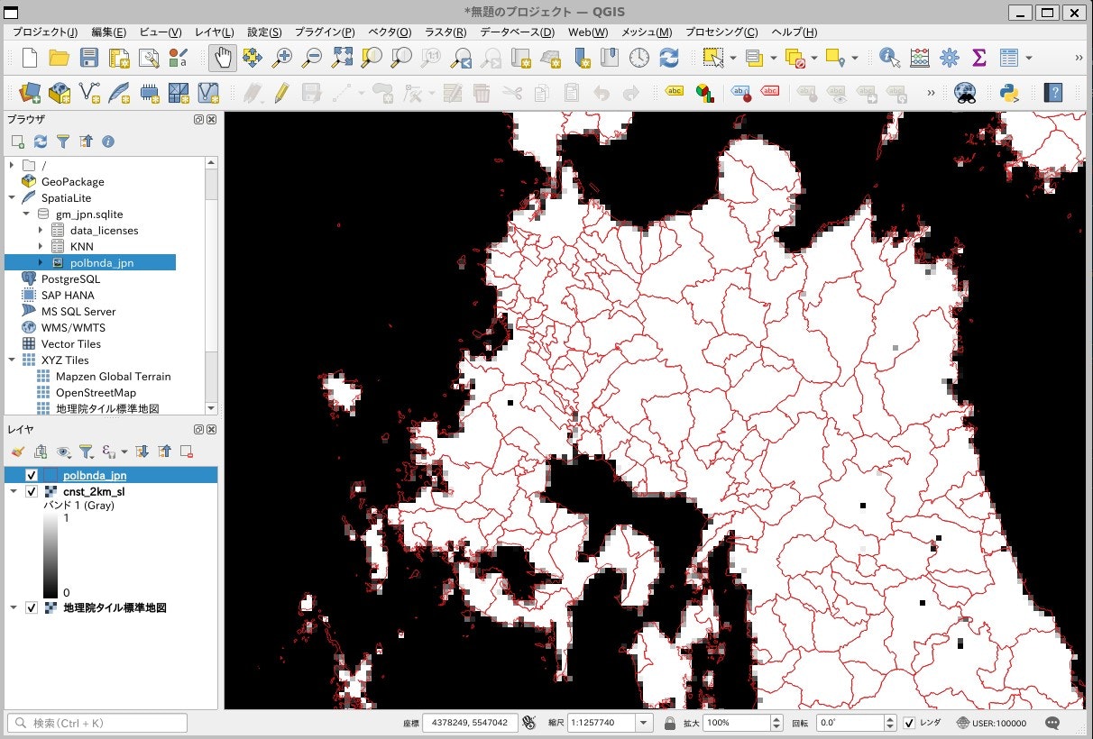
QGISに読み込んでみる
うまく投影変換されていることが確認できます。
結果
気候予測データセット2022の「日本域気候予測データ2㎞版」格子点データをGDALでラスタ化する際の投影パラメータは、
proj4文字列.
+proj=lcc +lat_1=30.0 +lat_2=60.0 +lon_0=80. +lat_0=0 +x_0=0 +y_0=0 +a=6371000 +b=6371000 +units=m +no_defs”
GeoTransFormパラメータ.
[4074196.5514666005,2000,0,7530619.71549598,0,-2000]
であると同定できました!
(個人)気候変化情報研究室では、できるだけ簡単に、将来、地域の気候がどのように変化するかを示すグラフ・地図を作成する方法を開発し、紹介しています。
興味のある方はぜひ読んでみてくださいね~。