I. Definition

Project Overview

The history of Open Source project is not so new, however, the faster new technologies are developing and the world is getting globalized, the more people engage in open source projects and the communities are growing. Thanks to the Internet, you are not necessary to be near around the communities to work with them. New innovative ideas are stimulated by people’s interaction across the world and developed as open source projects, e.g. OpenStack, Hadoop and TensorFlow.
But on the other hand, adapting open source products to business operation is not so easy. The development of open source products is very agile and engineers all over the world are always updating the source code. Because of the agility, open source products are always kind of beta version and have some bugs. As a result, there are many companies which offer professional services such as implementation, consulting and maintenance to help businesses utilize open source products.

Today, there are many companies packaging open source products as their service, e.g. Tera Data, HortonWorks, Mirantis and Red Hat. However, they are struggling to scale their business [1]. Even Red Hat, which has been one of the most successful Open Source Platform Business companies since they released their own Linux distribution called “Red Hat Linux” in 1994, the amount of earning is small comparing to other tech giants. For example, Amazon, which started a new cloud service “AWS” a decade ago, earned 12 billion dollars revenue only from AWS in 2016 [2], on the other hand, Red Hat earns just 2 billion dollars revenue from their total business in 2016 [3]. (But the amount is still much bigger than other open source business model based companies).

Problem Statement

Therefore, in order to find ways to maximize their business opportunities, a prediction model is to be created to “accurately identify which customers have the most potential business value for Red Hat” based on their characteristics and activities.”

In the data sets of this project, there are feature characteristics and a corresponding target variable “outcome” which is defined as yes/no binary flag. (It means, a customer’s activity has business value if the outcome of his/her activity is “yes”). Thus, it is necessary to create a binary prediction model which predicts what activities result in positive business outcome or not. As most of the features are categorical data, however, the data should be encoded into numerical values at first. Then, as supervisor data which has several features corresponding with the target “outcome” variable, the data set is passed to binary classification algorithm such as Decision Tree, Logistic Regression and Random Forest. Now, we have no idea which one should be used for this problem, as a result, these algorithms are going to be compared and the most appropriate one is chosen as a base model for the prediction model. When comparing the algorithms, the same metrics would be used to appropriately evaluate their result. After that, by using grid search method, the parameters for the algorithm will be optimized. Then, the prediction model is evaluated again and finally the optimized model is presented.

Metrics

To measure and evaluate the performance of the prediction results, Area under ROC Curve [4] is going to be used as this is a binary classification problem. In ROC curve, true positive rates are plotted against false positive rates. The closer AUC of a model is getting to 1, the better the model is. It means, a model with higher AUC is preferred over those with lower AUC.

II. Analysis

Data Exploration

Data set used in this project contains following data (You can find the data set at Kaggle project page [5]:

people.csv: This file contains people list. Each person in the list is unique identified by people_id and has his/her own corresponding characteristics.
act_train.csv: This activity file contains unique activities which are identified activity_id. Each activity is corresponding to its own activity characteristics. In the activity file, business value outcome is defined as yes/no for each activity.

Here, there are 8 types of activities. Type 1 activities are different from type 2-7 activities. Type 1 activities are associated with 9 characteristics, on the other hand, type 2-7 activities have only one associated characteristic. And also, in both csv files, except for “date” and “char_38” columns, all data type is categorical so it should be encoded before being processed by binary classification algorithms. Also, as the data sets are separated into 2 csv files, these files should be combined into a merged data set. After the merge, the shape of the training data set is (2197291, 55); 54 predictor features plus 1 target variable.
Exploratory Visualization
The following chart shows how many activities are performed in each month. According to the chart, “2022/10” has the maximum over 350,000 activities, on the other hand, “2022/07” has the minimum around 50,000 activities. Even though there are some difference in the number of activities among months, it shows no sign of upward trend.

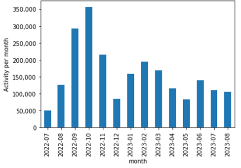
Fig. 1 Number of activities per month

The following chart shows how many people joined the community in each month. Even though there are some difference in the number of people join among months, it shows no sign of upward trend. However, as it shows the number of new people join at each month, it means, the number of community member is increasing month by month. According to the data set, the number of people in the data set is 189118 and the average number of people join per month is around 9000. Therefore, this community has more than 50% YoY growth in the number of community member. (It is amazing given the fact most of open source communities are struggling to gather people, however, it is also reasonable to think the similar number of people leave the community as well. But the data set includes no data to investigate it.)

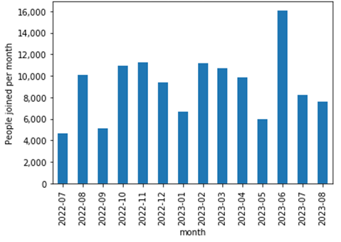
Fig. 2 Number of people join per month

The following chart is a very simple overview of the outcome of activities. It shows how many activities result in positive business value (“outcome” = 1) or not. As a result, 44% of activities has positive business impact.

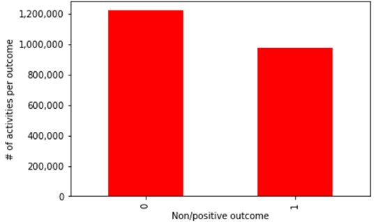
Fig. 3 Number of activities per outcome

The following chart is the histogram of community members based on the average outcome of their activities. Maximum is 1, minimum is 0 and the interval is 0.1. What is interesting here is the distribution is completely divided into 2 groups. Some people contribute to the community no matter what activities they do, but on the other hand, some people hardly contribute to the community. Therefore, finding people who has business value for the community is very critical for the prosperity of the community.

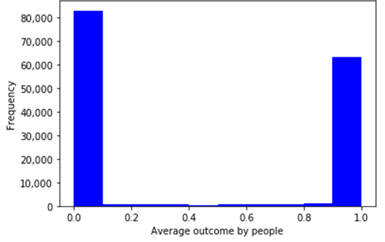
Fig. 4 Distribution of average outcome by people

In sum, there are 2 things I would like to mention here regarding to the charts. First, this community is a very active community in which constantly new members take part and many activities are performed, moreover, the numbers are really big. So it is reasonable to assume the samples in the dataset are not biased and represent the distribution of Red Hat’s community. Second, the above chart shows whether Red Hat community gains business value or not depends on who performs an activity. Therefore, the issue of this project stated in “Problem Statement” section is an appropriate target to be solved and creating a prediction model is a relevant approach.

Algorithms and Techniques

In order to predict which customers are more valuable for Red Hat business, a binary classification model should be created based on supervised algorithms such as decision tree, logistic regression and random forest tree by using training dataset which includes feature characteristics and a corresponding target variable “outcome” which is defined as yes/no binary flag.

In this project, 3 classification algorithms, Decision Tree [6], Logistic Regression [7] and Random Forest [8] are going to be compared at first. Each of them has its pros and cons, however, all of them can learn much faster than other supervise classification algorithms such as Support Vector Classifier [9]. The dataset of this project has more than 2 million samples with 50+ features, furthermore, 3 algorithms will be compared and grid search method will be used as well in the later phase of this project to optimize parameter. Therefore, choosing CPU and time efficient algorithms is reasonable choice.

These 3 algorithms are widely used for binary classification problem. Logistic Regression gives you a single linear decision boundary which divide your data samples. The pros of this algorithms are low variance and provides probabilities for outcomes, but as the con, it tends to be highly biased. On the other hand, Decision Tree gives you a non-linear decision boundary which divides the feature space into axis-parallel rectangles. This algorithm is good at handling categorical features and also visually intuitive how decision boundary divides your data but likely overfitting. Random Forest is actually an ensemble of decision trees which intends to reduce overfitting. It calculates a large number of decision trees from subsets of the data and combine the trees through a voting process. As a result, Random Forest is less overfitting models but makes it difficult to visually interpret.

Benchmark

This paper is based on the Kaggle project [5] and they set 50% prediction as benchmark. So in this paper, the benchmark is used as well.

III. Methodology

Implementation

The following flow chart shows the overview of the implementation process for creating a binary classification model. In case for reproducing this project, follow the below workflow and refer the code snippets which are cited on this paper.

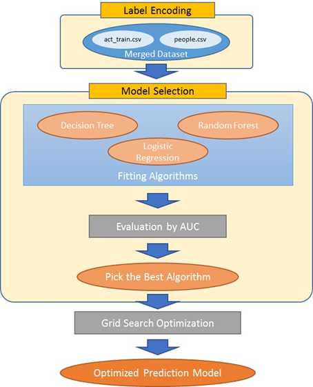
Fig. 5 Overview of implementation flow

Data Preprocessing

As the data sets prepared for this project are separated into 2 csv files, these files should be combined into a merged data set. The action csv file contains all unique activities and each unique activity has a corresponding people ID which shows who performed the activity. Thus, the relation between activity and people ID is one-to-many so that left join method is used for merging datasets on people ID by setting action csv as the left table. The below code is showing very brief overview of this merge implementation.

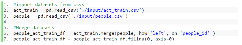
Fig. 6 Code Snippet: Merge people data to activity data

Then, since the most of columns in the dataset is categorical data as described in Data Exploration section, these categorical data should be encoded using label encoding algorithm [10]. Note that the samples in Fig. 7 contains just a few of columns in the dataset. As the dataset actually contains more than 50 features, most of columns are omitted intentionally.

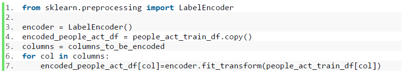
Fig. 7 Code Snippet: Encode dataset

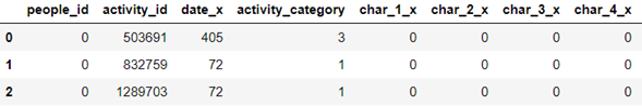
Fig. 8 Encoded date set samples

Finally, the dataset will be splitted into training and test sets in random order. In this project, 80% of the data will be used for training and 20% for testing.

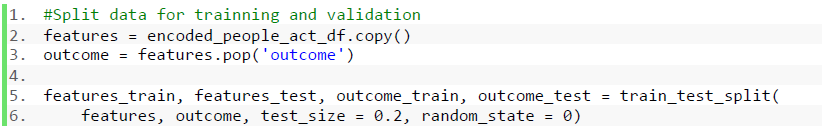
Fig. 9 Code Snippet: Split dataset

Model Selection

In the model selection phase, all parameters of the algorithms compared are set as default. In addition, in order to reduce the time to train algorithms, the training sample size is set to 100,000 samples.

For fitting algorithms and evaluating their predictions, the code below are implemented. Note that, where “classification_algorithm” represents supervised algorithm modules. Also, (features_train, outcome_train, features_test, outcome_test) are corresponding to the variables in Fig. 8 Code Snippet: Splitting dataset.

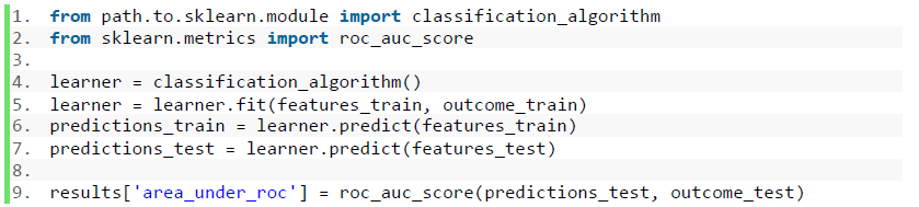
Fig. 10 Code Snippet: Fit and evaluate algorithm

IV. Results

Model Evaluation and Validation

For evaluation, Area under the ROC Curve [11] is used. AUC [4] is the size of area under the plotted curve. The closer AUC of a prediction model is getting to 1, the better the model is. Fig. 10 shows the code snippet for plotting ROC curve based on the prediction results by supervised algorithms. Note that, here "predictions_test" contains prediction results and "outcome_test" is the target score.

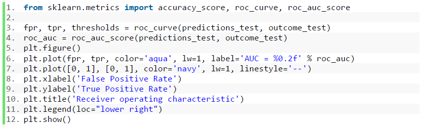
Fig. 11 Code Snippet: Plot ROC Curve

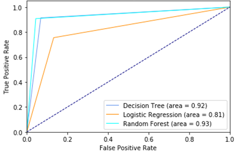
Fig. 12 ROC Curve and AUC of each algorithm

Refinement

Based on the result of the model selection phase, the most desirable prediction algorithm for this binary classification model is Random Forest, whose AUC value is 0.93.

Next, using grid search method [12], the binary classification model is going to be optimized further. In order to reduce the time for Grid Search, the training sample size is set to 100,000 samples. As optimized parameters, “n_estimator” and “min_sample_leaf” are chosen.

n_estimator: Grid Search parameter set 12, 24, 36, 48, 60
“n_esimator” is the number of trees to calculate. The higher number of trees, the better performance you get, but it makes the model learn slower.

min_samples_leaf: Grid Search parameter set 1, 2, 4, 8, 16
“min_samples_leaf” is the minimum number of samples required to be at a leaf node. The more leaf at a node, the less the algorithm catches noises.

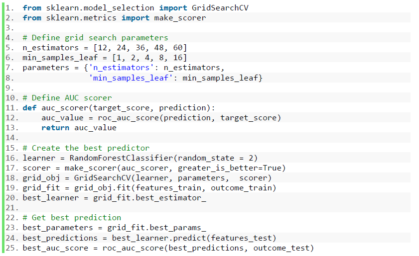
Fig. 13 Code Snippet: Grid Search Optimization

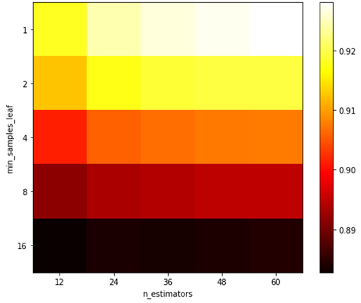
Fig. 14 Heat Map: Grid Search AUC Score

As a result of Grid Search, the best parameter for the model with the dataset is (“n_estimator”: 60, “min_samples_leaf”: 1). As you can see in Fig. 13 Heat Map, the more “n_estimator” gets bigger, the more the predictions are improved. On the other hand, the increase of “min_samples_leaf” are not effective, or rather, it decreases the prediction performance.

Justification

Finally, there is the optimized parameter set. Therefore, by training the model with the parameter sets and with the all 1,757,832 sample data, the best prediction result should be returned. As a result, the optimized model returned 0.993 AUC score and it is significantly greater than the benchmark (0.5).
In addition, to investigate if the model is robust and generalized enough (it means not overfitting), a new set of prediction results using the classification model was submitted to Kaggle competition (as this paper is based on Kaggle Project). For the submission, another dataset “act_test.csv” provided by Kaggle for the competition is used. Note that “act_test.csv” contains different data from “act_train.csv” which is used for model fitting. As a result, Kaggle evaluated the prediction made by the classification model and returned 0.863 AUC score. Therefore, the binary classification model is generalized enough to make good predictions based on unseen data.

V. Conclusion

Summary

The purpose of this project has been to build a binary classification prediction model for “identify which customers have the most potential business value for Red Hat”. Through the comparison of supervised classification algorithms and the optimization using Grid Search, finally, the best classification models, which is based on Random Forest Classifier, was built and scored 0.993 AUC score which is much higher than the benchmark score 0.5. In sum, using the prediction model, Red Hat can accurately predict which activities performed by its community members likely result in its positive business value. The prediction must be useful for planning its business strategies to maximize their return on investment.
In addition, as the code snippets for implementation is clearly stated throughout this paper, not just for reproducing the model for this specific issue but also it can be applied to similar binary classification issue with some code modification.

VI. Reference

Predicting Red Hat Business Value