日本統計学会公式認定統計検定準1級対応統計学実践ワークブック

が統計検定の準備だけでなく統計学の整理に役立つので、R, Pythonでの実装も試みた。

問17.1

データは下記から取得したがフォーマットが複雑なので手作業で準備した（本記事の末尾に記載）
- 総務省統計局 e-Stat 都道府県・市区町村のすがた（社会・人口統計体系）
  - 2017年度、「A1101_総人口【人】」「B1103_ 可住地面積【ｈａ】」
- 一般財団法人　自動車検査登録情報協会　自動車保有台数
  - 令和元年8月現在のデータがなく、令和二年2月現在のデータを用いた

R

df = read.csv('都道府県別_人口面積乗用車.csv')
dim(df)
head(df)

47 4
A data.frame: 6 × 4
都道府県    総人口   可住地面積 乗用車
<fct>   <int>   <int>   <int>
1   北海道   5320000 2237239 2818051
2   青森県   1278000 322970  734341
3   岩手県   1255000 371401  746817
4   宮城県   2323000 315488  1305508
5   秋田県   996000  320437  592573
6   山形県   1102000 288480  697137

df2 = df[! df$都道府県 %in% c('東京都', '大阪府', '神奈川県'), ]
dim(df2)

44 4

df2_1 = data.frame(c.ratio = df2$`乗用車` / df2$`総人口`, p.density = df2$`総人口` / df2$`可住地面積`)
head(df2_1)

A data.frame: 6 × 2
c.ratio p.density
<dbl>   <dbl>
1   0.5297088   2.377931
2   0.5746017   3.957024
3   0.5950733   3.379097
4   0.5619923   7.363196
5   0.5949528   3.108255
6   0.6326107   3.820022

model = lm(c.ratio ~ sqrt(p.density), data = df2_1)
summary(model)


Call:
lm(formula = c.ratio ~ sqrt(p.density), data = df2_1)

Residuals:
      Min        1Q    Median        3Q       Max 
-0.133071 -0.041664 -0.000793  0.051277  0.117539 

Coefficients:
                Estimate Std. Error t value Pr(>|t|)    
(Intercept)      0.74215    0.03161  23.479  < 2e-16 ***
sqrt(p.density) -0.05147    0.01033  -4.981 1.13e-05 ***
---
Signif. codes:  0 ‘***’ 0.001 ‘**’ 0.01 ‘*’ 0.05 ‘.’ 0.1 ‘ ’ 1

Residual standard error: 0.05825 on 42 degrees of freedom
Multiple R-squared:  0.3713,    Adjusted R-squared:  0.3564 
F-statistic: 24.81 on 1 and 42 DF,  p-value: 1.134e-05

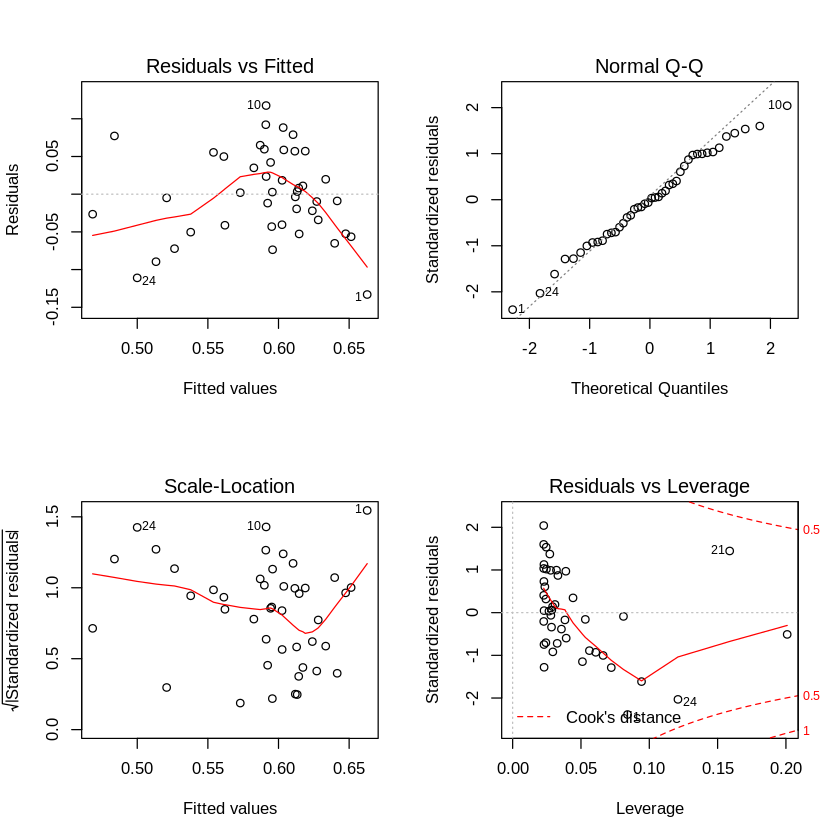
par(mfrow = c(2, 2))
plot(model)
par(mfrow = c(1, 1))

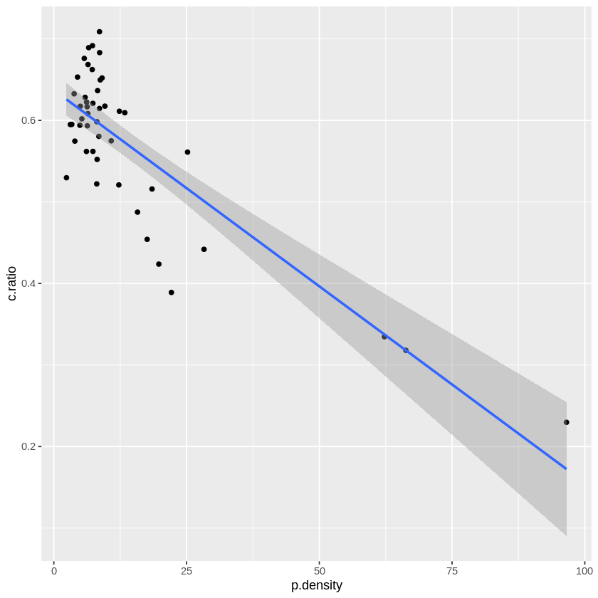
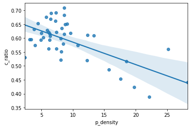
解答にある散布図と回帰曲線はいろいろ書き方があるがggplot2を使うのが簡単かつきれい、あと通常は信頼区間も示したほうがよいと思われる。

library(ggplot2)
df_1 = data.frame(c.ratio = df$`乗用車` / df$`総人口`, p.density = df$`総人口` / df$`可住地面積`)
ggplot(df_1, aes(x = p.density, y = c.ratio)) + geom_point() + geom_smooth(method = 'lm')

ggplot(df2_1, aes(x = p.density, y = c.ratio)) + geom_point() + geom_smooth(method = 'lm')

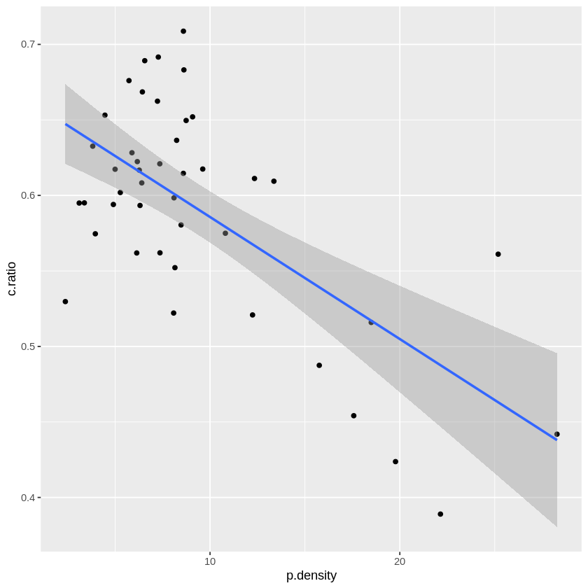
テキストとデータが若干異なるので図も異なるが趣旨としてはこの通り。

Python

import pandas as pd
import numpy as np
import statsmodels.formula.api as smf
from scipy import stats
import matplotlib.pyplot as plt

df = pd.read_csv('都道府県別_人口面積乗用車.csv')
df.head()

都道府県	総人口	可住地面積	乗用車
0	北海道	5320000	2237239
1	青森県	1278000	322970
2	岩手県	1255000	371401
3	宮城県	2323000	315488
4	秋田県	996000	320437

df2 = df[df['都道府県'].isin(['東京都', '大阪府', '神奈川県']) == False]
df2.shape

(44, 4)

df2_1 = pd.DataFrame({'c.ratio': df2['乗用車'] / df2['総人口'], 'p.density': df2['総人口'] / df2['可住地面積']})
df2_1.head()

c.ratio	p.density
0	0.529709
1	0.574602
2	0.595073
3	0.561992
4	0.594953

x = np.sqrt(df2['p.density'])
x = sm.add_constant(x)
y = df2['c.ratio']

results = smf.ols('c_ratio ~ np.sqrt(p_density)', data=df2_1).fit()
results.summary()

                  OLS Regression Results
Dep. Variable:    c_ratio       R-squared:          0.371
Model:            OLS           Adj. R-squared:     0.356
Method:           Least Squares F-statistic:        24.81
Date:   Sun, 26 Jul 2020        Prob (F-statistic): 1.13e-05
Time:             10:36:04      Log-Likelihood:     63.679
No. Observations: 44            AIC:                -123.4
Df Residuals:     42            BIC:                -119.8
Df Model:         1     
Covariance Type:    nonrobust       
                   coef    std err t       P>|t| [0.025  0.975]
Intercept      0.7421  0.032   23.479  0.000  0.678  0.806
np.sqrt(p_density) -0.0515 0.010   -4.981  0.000  -0.072 -0.031
Omnibus:       0.516    Durbin-Watson:    1.078
Prob(Omnibus): 0.772    Jarque-Bera (JB): 0.639
Skew:          -0.104   Prob(JB):         0.726
Kurtosis:      2.447    Cond. No.         12.1


Warnings:
[1] Standard Errors assume that the covariance matrix of the errors is correctly specified.

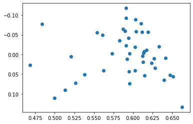
ax = plt.subplot()
ax.invert_yaxis()
ax.scatter(result.fittedvalues, result.fittedvalues - df2_1['c_ratio'])

stats.probplot(stats.zscore(result.fittedvalues - df2['c_ratio']), dist="norm", plot=plt);

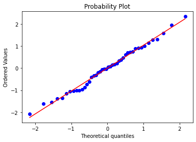
テキスト、Rとちょっと違う、、、

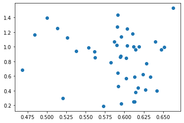
plt.scatter(result.fittedvalues, np.sqrt(np.abs(stats.zscore(result.fittedvalues - df2['c_ratio']))))

sm.graphics.influence_plot(results, size = 1);

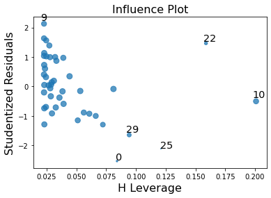
番号がずれているがプロットは正しそう。
解答にある図　seaborn を用いた

import seaborn as sns
df_1 = pd.DataFrame({'c_ratio': df['乗用車'] / df['総人口'], 'p_density': df['総人口'] / df['可住地面積']})
sns.regplot(x="p_density", y="c_ratio", data=df_1)

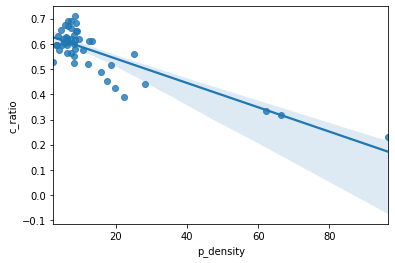
sns.regplot(x="p_density", y="c_ratio", data=df2_1)

都道府県別_人口面積乗用車.csv

都道府県,総人口,可住地面積,乗用車
北海道,5320000,2237239,2818051
青森県,1278000,322970,734341
岩手県,1255000,371401,746817
宮城県,2323000,315488,1305508
秋田県,996000,320437,592573
山形県,1102000,288480,697137
福島県,1882000,421711,1229236
茨城県,2892000,397512,2000193
栃木県,1957000,298276,1348806
群馬県,1960000,227936,1389173
埼玉県,7310000,258464,3230250
千葉県,6246000,355433,2836551
東京都,13724000,142143,3152966
神奈川県,9159000,147093,3065153
山梨県,823000,95438,562220
新潟県,2267000,453532,1399511
富山県,1056000,184282,713894
石川県,1147000,139182,730058
長野県,2076000,322552,1387924
福井県,779000,107729,516016
岐阜県,2008000,221113,1309297
静岡県,3675000,274948,2239573
愛知県,7525000,298821,4222263
三重県,1800000,205918,1169327
滋賀県,1413000,130722,812401
京都府,2599000,117382,1010972
大阪府,8823000,133058,2805443
奈良県,1348000,85553,657131
和歌山県,945000,111506,548525
兵庫県,5503000,278293,2331794
鳥取県,565000,90083,348468
島根県,685000,129888,412318
岡山県,1907000,221871,1172093
広島県,2829000,231109,1473531
山口県,1383000,170697,827588
徳島県,743000,101035,461360
香川県,967000,100559,597098
愛媛県,1364000,167326,753155
高知県,714000,116311,401196
福岡県,5107000,276153,2634631
佐賀県,824000,133561,512857
長崎県,1354000,167496,706950
熊本県,1765000,279626,1047274
大分県,1152000,179893,700764
宮崎県,1089000,184988,684196
鹿児島県,1626000,331288,965856
沖縄県,1443000,116902,881983

『統計検定準1級対応統計学実践ワークブック』をR, Pythonで解く～第17章回帰診断法～

問17.1

R

Python