概要
AIトップカンファレンスの一つ、AAAI(Association for the Advancement of Artificial Intelligence) の研究トレンドを論文タイトルから分析してみます。
(時期的にCVPRで試したかったですが、後述のAPIで2024年分が取得できなかったので、データが揃っていたAAAIを選定しています)
2020~2024年の5年間を対象に分析した結果、
- language model や diffusion model などの生成モデル系
- federated learning
- point cloud
- backdoor attack
などに関する研究が増加傾向にあるようです。
はじめに
近年、様々な分野で研究開発が急速に発展しており、技術トレンドのキャッチアップが難しくなってきています。
そこで今回は、論文タイトルを自然言語処理を用いて分析し、効率的なトレンド推定を図ります。
Deep Learningは使わず、形態素解析・熟語の出現回数などから導出してみます。
検証条件
データの可視化などを勘案し、Jupyter Notebook (*.ipynbファイル)形式で実施します。
- 環境、ライブラリ
- python 3.10
- inflection==0.5.1
- matplotlib==3.9.0
- networkx==3.3
- pandas==2.2.2
- requests==2.32.3
- scipy==1.14.0
- spacy==3.7.5
- tqdm==4.66.4
- ipykernel==6.29.4
事前準備
今回は形態素解析にspaCyを使用します。
解析を始める前にターミナルで下記コマンドを実行し、英語用辞書をダウンロードしておきます (参考)。
python -m spacy download en_core_web_sm
データの用意
学会や著者などのメタデータつきで論文タイトルを取得できる、dblp APIにて収集します。
データは商用利用可能なライセンスで公開されています (参考)。
dblp APIの利用に際し、dblpのサーバー側に負荷をかけないよう一定時間おきにアクセスします。
時間間隔の推奨がAPIに記載されていなかったため、念のため10秒間隔にしています。
(参考:arxiv APIはアクセス間隔3秒以上を推奨 arXiv API User's Manual)
import re
import time
from typing import Any

import pandas as pd
import requests
from tqdm.auto import tqdm

DBLP_API_URL = "https://dblp.org/search/publ/api"  # DBLP APIのURL
SLEEP_TIME = 10  # API処理 待機時間[sec]
YEAR_LIST = [2020, 2021, 2022, 2023, 2024]  # 取得対象年


def run_dblp_api(params: dict[str, str | int]) -> dict[str, Any]:
    _response = requests.get(DBLP_API_URL, params=params)
    response = _response.json()
    return response


# APIクエリパラメータ
query_params = {
    "format": "json",
}
# 取得するメタデータ
info_col = ["title", "year", "type", "key"]
paper_info_dic = {k: [] for k in info_col}
for year in tqdm(YEAR_LIST):
    query_params["q"] = f"streamid:conf/aaai: year:{year}:"  # AAAIに関する指定yearの論文情報を取得するクエリ
    query_params["f"] = 0
    query_params["h"] = 1
    response = run_dblp_api(query_params)
    total_num = int(response["result"]["hits"]["@total"])

    for f in range(0, total_num+1, 1000):
        query_params["f"] = f
        query_params["h"] = 1000
        response = run_dblp_api(query_params)
        # 論文情報の取得
        for paper in response["result"]["hits"]["hit"]:
            if all([col in paper["info"] for col in info_col]):
                for col in info_col:
                    paper_info_dic[col].append(paper["info"][col])

        time.sleep(SLEEP_TIME)

paper_df = pd.DataFrame(paper_info_dic)
paper_dfの内容はこのような形式になります。

type列をみると、Conference and Workshop Papersの他にEditorshipが含まれています。Editorshipは学会特集号などを指すため、研究論文とは異なり分析にはノイズになる可能性が高いです。
以下の処理でAPI取得結果を整形します。
def remove_parentheses(text: str) -> str:
    """ 括弧を含む文字列を除去

    Args:
        text (str): 対象文章

    Returns:
        str: 除去結果
    """
    pattern = r"\(.*?\)"
    result = re.sub(pattern, "", text)
    return result

# ノイズ除去
paper_df = paper_df[paper_df["type"]=="Conference and Workshop Papers"]
paper_df["key_conference"] = paper_df["key"].str.split("/").str[1]  # AAAI本会議と異なる論文が混じることがあるため、フィルタリング処理
paper_df = paper_df[paper_df["key_conference"]=="aaai"]

# クリーニング
paper_df["year"] = paper_df["year"].astype("int")  # 年情報をstr->intへ
paper_df = paper_df[~paper_df["title"].str.lower().str.contains("student abstract")]
paper_df["title"] = paper_df["title"].apply(remove_parentheses)
paper_df["title"] = paper_df["title"].str.replace("-", "_")  # 後述の形態素解析をしやすいよう、-記号を_記号に置換
paper_df.reset_index(drop=True, inplace=True)
以上の処理で、合計10,046件の論文を収集できました。
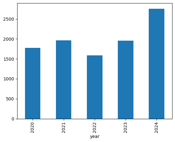
年別の件数を確認すると、2022年から2024年にかけて1,000件以上増加しているようです。
paper_df["year"].value_counts().sort_index().plot.bar()
トレンドワード推定
近年増加傾向にあるワード≒トレンドワードと捉え、論文タイトルからbi-gram(2単語の熟語)の抽出、年別の出現回数を比較します。
論文タイトルからワード(bi-gram)抽出
形態素解析ライブラリ spacy を使用します。
spacyで品詞を判定し、"NOUN"(名詞), "PROPN"(固有名詞)を対象にbi-gram化します。
import re
from collections import Counter, OrderedDict
from itertools import combinations

import inflection
import matplotlib.pyplot as plt
import networkx as nx
import numpy as np
import pandas as pd
import spacy
from scipy.sparse import dok_matrix
from scipy.stats import linregress
from tqdm.auto import tqdm

# 形態素解析器の用意
nlp = spacy.load("en_core_web_sm")


def get_ngram(
    texts: list[str],
    gram_num: int = 2,
    stop_words: list[str] = [],
    target_pos: list[str] = [],
) -> list[str]:
    """熟語(n-gram)を取得。
    gram_numで指定した数のトークンを連結し、熟語とする。

    Args:
        texts (list[str]):
            処理対象文章.
        gram_num (int, optional):
            連結するトークンの数。デフォルトは2。
        stop_words (list[str]], optional):
            ストップワードのリスト。デフォルトは [].
        target_pos (list[str]], optional):
            抽出したい品詞がある場合に使用。
            [] の場合はすべての品詞を取得。デフォルトは [].

    Returns:
        List[str]:
            n-gramのリスト。
    """

    pattern = r"o+"
    join_str = "_"

    results = []
    for text in tqdm(texts):
        pos_str = ""
        tokens = []
        n_grams = []
        doc = nlp(text)
        if target_pos:
            for token in doc:
                tokens.append(token.text)
                if (token.pos_ in target_pos) & (token.text not in stop_words):
                    pos_str += "o"
                else:
                    pos_str += "x"
        else:
            for token in doc:
                tokens.append(token.text)
                if token.text not in stop_words:
                    pos_str += "o"
                else:
                    pos_str += "x"

        for match in re.finditer(pattern, pos_str):
            start = match.start()
            end = match.end()
            length = end - start
            if length >= gram_num:
                for s in range(start, end - gram_num + 1):
                    n_grams.append(
                        join_str.join(
                            [
                                inflection.singularize(w)
                                for w in tokens[s : s + gram_num]
                            ]
                        ).lower()
                    )
        results.append(n_grams)

    return results


stop_words = list(nlp.Defaults.stop_words)
title_words = get_ngram(
    paper_df["title"].to_numpy(),
    stop_words=stop_words,
    target_pos=["NOUN", "PROPN"],
)

# 論文ごとに重複ワードを除去
title_words = [list(OrderedDict.fromkeys(x)) for x in title_words]

# 抽出したワードのユニーク数
len(np.unique(np.concatenate(title_words)))
21575
全部で21,575件のワードを取得できました。
こんな形で論文タイトルからワードを抽出しています。
| 論文タイトル | 抽出ワード |
|---|---|
| Results on a Super Strong Exponential Time Hypothesis | super_strong, strong_exponential, exponential_time, time_hypothesis |
| Adversarial_Learned Loss for Domain Adaptation | adversarial_learned_loss, domain_adaptation |
| Minecraft as a Platform for Project_Based Learning in AI | project_based_learning |
増加傾向にあるワードの導出
ワード出現傾向を単回帰モデルに適用し、増減傾向を定量化します。
出現傾向は、論文数自体が年々増加している点を考慮し、出現回数を各年の総論文数でスケーリングした値を使用します。各年における割合(話題性)でトレンドを推定する形になります。
# 年別の出現回数集計
year_count_list = []
for year in YEAR_LIST:
    year_words = np.array(title_words, dtype=object)[paper_df["year"] == year]
    year_words = np.concatenate(year_words)
    count = Counter(year_words)
    year_count_list.append(
        pd.DataFrame(index=count.keys(), columns=[year], data=count.values())
    )
year_count_df = pd.concat(year_count_list, axis=1).fillna(0)
# スケーリング
year_rate_df = year_count_df.copy()
for year in YEAR_LIST:
    year_rate_df[year] /= np.sum(paper_df["year"] == year)
    year_rate_df[year] *= 100
増加傾向は、近年のトレンド推定・短期変動によるノイズ除去を行えるよう、短期・中期の2期間を組み合わせて導出します。
- 短期(近年のトレンド推定):2023 ~ 2024年
- 中期(短期変動によるノイズ除去):2020 ~ 2024年
各期間における変動を単回帰モデルに適用し、傾きを求めます。
def calc_slope(
    year_rate_df: pd.DataFrame,
    year_list: list[int],
    ) -> pd.DataFrame:
    """回帰

    Args:
        year_rate_df (pd.DataFrame): ワードx年別の出現割合
        year_list (list[int]): 算出期間

    Returns:
        pd.DataFrame: ワード別の単回帰モデル傾き
    """
    slope_dict = {x:np.nan for x in year_rate_df.index}
    for i, word_year_rate in tqdm(
        zip(year_rate_df.index, year_rate_df[year_list].to_numpy()),
        total=len(year_rate_df),
    ):
        slope, _, _, _, _ = linregress(year_list, word_year_rate)
        slope_dict[i] = slope

    slope_df = pd.DataFrame(
        data=slope_dict.values(),
        index=slope_dict.keys(),
        columns=["slope"]
    )
    return slope_df

# 短期:2023~2024年
y2_slope_df = calc_slope(
    year_rate_df,
    range(2023, 2024 + 1)
)

# 中期:2020~2024年
y5_slope_df = calc_slope(
    year_rate_df,
    range(2020, 2024 + 1)
)
顕著に増加している(傾きが正に大きい)ワードを平均+3σで抽出し、短期・中期の両方で抽出したワードを確認してみます。
y2_high_slope_th = y2_slope_df["slope"].std() * 3 + y2_slope_df["slope"].mean()
y2_high_slope_words = y2_slope_df["slope"][
    y2_slope_df["slope"] >= y2_high_slope_th
].sort_values(ascending=False)

y5_high_slope_th = y5_slope_df["slope"].std() * 3 + y5_slope_df["slope"].mean()
y5_high_slope_words = y5_slope_df["slope"][
    y5_slope_df["slope"] >= y5_high_slope_th
].sort_values(ascending=False)

# 短中期で顕著なワード
both_high_slope_words = list(set(y5_high_slope_words.index) & set(y2_high_slope_words.index))

len(both_high_slope_words)
28
# 短中期で顕著なワード&直近2年の傾きTop10
sorted_both_high_words = y2_slope_df.loc[both_high_slope_words]["slope"].sort_values(ascending=False).index
year_rate_df.loc[sorted_both_high_words[:10]].T.plot.line(marker="o")
plt.legend()
plt.show()
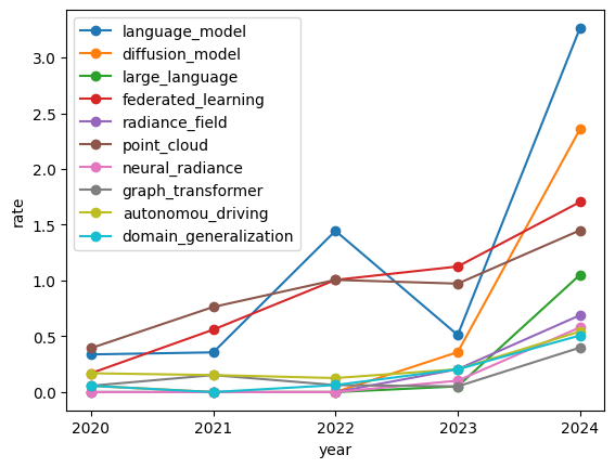
language_model, diffusion_modelといった生成モデルに関するワードが2023-2024年にかけて約2%増加しています。
また、連合学習の意である federated_learningは2020年から継続して増加しています。
language_modelは2022年も一時的に増加しているため、同時に出現するワードを2022年と2024年で比較し話題の変化をみてみます。
# 2022年
target_word = "language_model"
year_title_words = np.array(title_words, dtype="object")[paper_df["year"]==2022]
target_contain_words = np.concatenate([w for w in year_title_words if target_word in w])
Counter(target_contain_words).most_common(5)
[('language_model', 23),
 ('coding_manual', 1),
 ('building_better', 1),
 ('better_language', 1),
 ('code_understanding', 1),
 ('enhanced_story', 1)]
# 2024年
target_word = "language_model"
year_title_words = np.array(title_words, dtype="object")[paper_df["year"]==2024]
target_contain_words = np.concatenate([w for w in year_title_words if target_word in w])
Counter(target_contain_words).most_common(5)
[('language_model', 90),
 ('large_language', 29),
 ('model_evaluation', 2),
 ('model_based', 2),
 ('vision_language', 2)]
2022年は共起回数が1回のワードが多いためユニークな話題のようですが、2024年はlarge_languageの共起が多くなっています。
Large Language Model(LLM)の存在自体は2020年頃からありましたが、明示的に大規模モデルを指す研究が増えているようです。
共起分析
増加傾向であったワードのうち、他のワードと紐づきやすいワードを主要トレンド技術・トピックと仮定し、共起分析もしてみます。
前節で求めた増加ワード同士の共起ネットワークを作成し、中心媒介性が上位のワードを確認します。
def count_cooccurrences(text_words: list[list[str]], vocab: list[str]) -> dok_matrix:
    """ワードの共起回数をカウント

    Args:
        text_words (list[list[str]]): 各文章のワード
        vocab (list[str]): 集計対象の語彙

    Returns:
        dok_matrix: 共起行列
    """
    vocab_index = {word: idx for idx, word in enumerate(vocab)}
    cooccurrence_matrix = dok_matrix((len(vocab), len(vocab)), dtype=int)

    for title_n_gram in tqdm(text_words):
        for word1, word2 in combinations(title_n_gram, 2):
            if word1 in vocab_index and word2 in vocab_index:
                idx1, idx2 = vocab_index[word1], vocab_index[word2]
                cooccurrence_matrix[idx1, idx2] += 1
                cooccurrence_matrix[idx2, idx1] += 1  # 対称行列
    return cooccurrence_matrix


def create_cooccurrence_network(
    cooccurrence_matrix: dok_matrix, vocab: list[str], count_th: int = 0
) -> nx.Graph:
    """共起ネットワーク作成

    Args:
        cooccurrence_matrix (dok_matrix): 共起行列
        vocab (list[str]): 集計対象の語彙
        count_th (int, optional): グラフ化する共起回数の最小閾値. Defaults to 0.

    Returns:
        nx.Graph: 共起ネットワーク
    """
    G = nx.Graph()
    for (i, j), weight in cooccurrence_matrix.items():
        if weight > count_th:  # 閾値を設定する場合はここで調整
            G.add_edge(vocab[i], vocab[j], weight=weight)
    return G


# 2024年の共起回数集計
recent_title_words = np.array(title_words, dtype="object")[paper_df["year"]==2024]
cooccurrence_matrix = count_cooccurrences(recent_title_words, both_high_slope_words)
# 共起ネットワーク作成
G = create_cooccurrence_network(cooccurrence_matrix, both_high_slope_words)

# 媒介中心性計算
bc = nx.betweenness_centrality(G, endpoints=True)
# 上位(IQR*1.5以上)ワード抽出
p75 = np.percentile(list(bc.values()), 75)
p25 = np.percentile(list(bc.values()), 25)
th = p75 + 1.5*(p75-p25)

for k, v in sorted(bc.items(), key=lambda x: -x[1]):
    if v >= th:
        print(str(k) + ": " + str(v))
point_cloud: 0.32105263157894737
backdoor_attack: 0.3026315789473684
diffusion_model: 0.25526315789473686
Lidarに代表されるpoint_cloud、モデル攻撃手法であるbackdoor_attackのワードが他の増加ワードと共起しやすいようです。
backdoor_attackは特定のモデルに限らずケアすべき話題であるため、機械学習サービスの運用に向けて今後も注目していきたいです。
最後まで読んでいただき、ありがとうございました!
今後も機械学習の活用を始め、開発環境やシミュレーションなど幅広く技術情報発信をしていく予定です!
最後になりますが、本記事の内容に誤りなどあれば、コメントにてご教授お願いいたします。