時系列データ向けの表現学習「T-Rep (ICLR2024論文)」の紹介

概要

時系列データ向けの表現学習手法「T-Rep: Representation Learning for Time Series using Time-Embeddings」 (ICLR2024) の論文、公式リポジトリを読んだので備忘録を兼ねて紹介します。
本手法は多変量の時系列データに対応しており、表現学習時に複数のPretextタスクを導入することで異常検出や分類・予測に寄与する汎用的な特徴量を獲得しています。
時系列表現(representation)はタイムスタンプ単位で出力できるため、point-wiseな異常検出であったり、window単位で集約することでsegment-wiseな分類や異常検出も可能な手法です。

記事の後半では公式チュートリアルを参考に、多変量時系列データの分類を試してみます。

arxiv

Github

先行研究や数式の詳細は割愛してます。
論文の解説記事を書くことが初めてなので、至らない点・誤りなどあればコメントにてご指南ください。

モデル構造

T-Repモデルは以下の3つのモジュールから構成されています。

Linear Projection LayerとTime-Embedding Moduleでそれぞれ多変量時系列データとタイムスタンプを変換し、Dilated 1D-CNNで短期・長期的な時系列表現を集約します。

1. Linear Projection Layer
   • 次元数Cの多変量をタイムスタンプ単位で集約し、次元数Fに射影
   • input : 多変量時系列データ $[x_1, \dots, x_T] \in \mathbb{R}^{C}$
   • output : 射影ベクトル $[u_1, \dots, u_T] \in \mathbb{R}^{F}$
2. Time-Embedding Module
   • タイムスタンプ$t$から時系列に関連する特徴(トレンド、周期性、分布シフトなど)を学習
     • 先行研究の Time2Vec を使用し、sin波による周期的な特徴と線形な特徴を組み合わせ
   • input : タイムスタンプ $[0, 1, \dots, T-1]$
   • output : 時間埋め込み $[τ_1, \dots, τ_T] \in \mathbb{R}^{F'}$
3. Dilated 1D-CNN Encoder
   • 複数のDilated 1D-CNNブロック(Residual付き)で構成。デフォルトでは11ブロック。
   • input : 射影ベクトル$u$ と 時間埋め込み$τ$ をチャネル方向に結合 $[,u_1 ,|, \tau_1,; \dots,; u_T ,|, \tau_T] \in \mathbb{R}^{F+F'}$
   • output : 時系列表現 $[z_1, \dots, z_T]$

Pretextタスク

Pretextタスクとは、データ自体から生成した疑似ラベルを基に、下流タスクに役立つ汎用的な特徴を学習させるものです。
例えば表現学習においては、以下に代表するようなPretextタスクがあります。

• Encoder-Decoderによる入力データの再構成学習
• Encoderのみ用いたPositive-Negativeペアの対照学習

時系列データでは「隣接するWindowは類似するはず」という仮定のもと対照学習用のPosi-Negaペアを用意する手法が一般的です。 一方で、これらのペアは周期的・不規則に繰り返すパターンを捉えるには不向きである点、細かい時間依存関係を学習するのが難しい点をT-Rep論文では指摘しています。

T-Repでは以下4つのPretextタスクで学習することで、上記課題を対処しています。
1,2 は先行研究 TS2Vec を踏襲しており、3, 4が新規提案タスクになります。

1. Instance-wise contrasting
2. Temporal contrasting
3. Time-embedding divergence prediction
4. Time-embedding-conditioned forecasting

基本的には下図の流れで表現ベクトル $z$、時間埋め込み $τ$を生成し、各PretextのLossを算出します。
各Lossは合計1になるよう重みづけして集約され、デフォルトでは 各 0.25 で均等な配分になっています。

学習時はDilated 1D-CNNへ入力する前にランダムなタイムスタンプでマスキングしている点が重要で、元は同じinstanceであっても異なるcontextを持つよう誘導しています。
これにより、時系列構造に対するロバスト性を向上・対照学習時のPositiveデータサンプリングバイアス低減を図っています。

Instance-wise contrasting

• 目的：instance(サンプル)間の識別性向上
• タスク：instance間で対照学習
  • 重複していた箇所の表現ベクトル $z$ をバッチ内のinstance間で比較
  • 同じinstance同士はpositiveペア、異なるinstance同士はnegativeペアとする

Temporal contrasting

• 目的：時間軸に沿った一貫性向上
• タスク：タイムスタンプ間で対照学習
  • 重複していた箇所の表現ベクトル $z$ を同じinstanceのタイムスタンプ間で比較
  • 同じタイムスタンプ同士はpositiveペア、異なるタイムスタンプ同士はnegativeペアとする

Time-embedding divergence prediction

• 目的：表現ベクトル $z$ の空間構造に時間の概念を統合させる
• タスク：表現ベクトル $z$ から、元の時間埋め込み $τ$ の情報を復元
  • 記号の定義：
    • $z_{i,t}$, $z'_{j,t'}$：異なるinsetance $i, j$且つ、異なるタイムスタンプ $t, t' (t≠t')$の表現ベクトル を用意
    • $τ_t$, $τ_{t'}$：タイムスタンプ $t, t'$ に対応する時間埋め込み
    • $g_1$ ：表現ベクトルの差分から距離尺度を回帰するモジュール
      • input:表現ベクトルの次元, output:1次元。パラメータは学習対象
    • $JSD$：Jensen-Shannon divergence(JSD)
    • $MSE$：Mean Squared Error
  • ランダムサンプリングした複数の $i, j, t, t'$ を対象に

    MSE(g_1(z_{i,t} - z'_{j,t'}) - JSD(τ_t || τ_{t'}))
    

    を最小化
  • 時間埋め込みの差分をノルムではなくJSDで算出する意図は、時間軸を考慮させるため
    • 例：時刻 00:00:00 (HH:MM:SS) に対し 01:01:01 と 03:00:00 を比較した場合、ノルムでは両者とも差分 3.0 となり違いを判断できない

Time-embedding-conditioned forecasting

• 目的：時間埋め込みに予測情報を組み込み、欠損データに対する頑健性向上
• タスク：現時点の表現ベクトル $z_t$ と 別時点の時間埋め込み $τ_{t+Δ}$ から、別時点の表現ベクトル $z_{t+Δ}$ を予測
  • 記号の定義：
    • $z_{i,t}$：insetance $i$ 、タイムスタンプ $t$ における表現ベクトル
    • $τ_t$：タイムスタンプ $t$ に対応する時間埋め込み
    • $t+Δ$：予測先のタイムスタンプ
      • $∆$ は $[-∆_{max}, ∆_{max}]$の範囲で一様サンプリング。$Δ_{max}$ はハイパーパラメータ
    • $c1, c2$：単一のinstanceから取得した2種のcontextからランダムサンプリング。同じcontextになることもある
    • $g_2$：表現ベクトルと時間埋め込みから表現ベクトルを回帰するモジュール
      • input:表現ベクトル次元+時間埋め込み次元, output:表現ベクトル次元。パラメータは学習対象
  • ランダムサンプリングした複数の $t, Δ$ を対象に

    MSE(g_2([z^{(c1)}_{i,t} τ_{t+Δ}]^T) - z^{(c2)}_{i,t+Δ})
    

    を最小化

評価

論文中ではT-Repで獲得した時系列表現の評価として、モデルで獲得した時系列表現をもとにした下流タスク(異常検出・分類・予測)の精度検証、欠損データに対する頑健性を先行研究と比較しています。
以降では各タスクにおけるT-Repの実施条件のみ簡単に説明します。その他手法の実験条件は論文のAPPENDIXをご参照ください。

異常検出

Yahooデータセットはpoint-wiseな異常、Sepsisデータセットはsegment-wiseな異常を対象にしたデータセットです。

point-wiseな異常検出に対しては、pretext中にランダムマスキングしながら表現ベクトルを獲得している点を利用しています。 具体的には、「検出対象のタイムスタンプ $t$ のみマスクした場合」と「全てマスクしていない」場合の 表現ベクトル $z_t$ の差分を集計し、外れ値＝異常データと定義します。

• マスク別の表現ベクトル取得コード

  # https://github.com/Let-it-Care/T-Rep/blob/d624998e30b34f365649b13c1cade7c54c41687f/tasks/anomaly_detection.py#L93
  
  def encode_data_wm(data):
        return model.encode(
                data.reshape(1, -1, 1),
                mask='mask_last',  # 最終タイムスタンプのみマスクあり
                causal=True,  # causal=True：過去のタイムスタンプのみ参照
                sliding_length=1,
                sliding_padding=200,
                batch_size=256,
            ).squeeze()
  
  # マスクなし
  def encode_data_wom(data):
      return model.encode(
              data.reshape(1, -1, 1),
              causal=True,
              sliding_length=1,
              sliding_padding=200,
              batch_size=256,
          ).squeeze()
  

Sepsisは時間軸方向にの表現ベクトルを max pooling で集約し、RBFカーネルのSVMで教師あり学習しています。TS2Vecも表現ベクトル獲得以降は同様の枠組みで実施しているようです。

分類

T-Repは時系列表現をタイムスタンプ単位、インスタンス単位(時間軸方向にmax pooling)の両方で実施可能です。
論文中のベンチマークでは中期的な特徴集約を狙い、移動窓で部分的にmax poolingし結合したものをRBFカーネルのSVMに入力しています。

• インスタンス、window単位の集約コード

  # https://github.com/Let-it-Care/T-Rep/blob/d624998e30b34f365649b13c1cade7c54c41687f/tasks/classification.py#L9
  
  # インスタンス単位の集約
  if encoding_protocol == 'full_series':
      # 'full_series' encodes time series in 1 vector (no temporal dimension). This is the default and simplest setting.
      # It should be sufficient for most applications, but for maximum performance use 'timedim'.
      assert train_labels.ndim == 1 or train_labels.ndim == 2
      train_repr = model.encode(train_data, encoding_window='full_series' if train_labels.ndim == 1 else None)
      test_repr = model.encode(test_data, encoding_window='full_series' if train_labels.ndim == 1 else None)
  # window単位の集約
  elif encoding_protocol == 'timedim':
      # 'timedim' encodes time series at a user-specified temporal granularity, resulting in higher-dimensional representations
      # to classify, but more easily separable. This can boost performance, but it more computationally expensive and requires
      # tuning hyper-parameter k.
      assert train_data.shape[1] == test_data.shape[1]
      T = train_data.shape[1]
      k = 10
      w = (T // k) if T > k else 1
      train_repr = model.encode(train_data, encoding_window=w if train_labels.ndim == 1 else None)
      test_repr = model.encode(test_data, encoding_window=w if train_labels.ndim == 1 else None)
  
      train_repr = train_repr.reshape(train_repr.shape[0], -1)
      test_repr = test_repr.reshape(test_repr.shape[0], -1)
  

予測

過去L点分の時系列表現をもとに、将来時点の時系列データを予測します。ベンチマークでは時系列表現をリッジ回帰に入力することで、回帰モデルを構築しています。

欠損データに対する頑健性

Pretext時にランダムマスキングを実施しているため、エンコード時に入力データが一部欠損していても他のタイムスタンプから時系列表現を獲得できるようです。右側のグラフでは50%欠損していても未欠損と同等の分類精度が出ています。
(所感：欠損の仕方が、point単位なのかsegment単位なのかで影響度合いが大きく変わりそう。本評価時の欠損方法がどちらなのかは分からず。)

アブレーションスタディ(Pretextタスク,アーキテクチャの重要性)

予測・異常検知タスクを対象に、T-Repで新規提案した2種のPretextタスクや時間埋め込みモデル構造の効果を検証しています。
どちらも提案したPretextタスク・モデル構造において精度が高かったようです。

実際に検証してみる

公式リポジトリのREADME.mdやチュートリアルnotebookを参考に、多変量時系列データの分類をしてみます。

検証条件
データの可視化などを勘案し、Jupyter Notebook (*.ipynbファイル)形式で実施します。

• 環境、ライブラリ
  • python: 3.10
  • CUDA Version: 12.2
  • GPU: NVIDIA RTX A6000
  • torch == 2.5.1
  • umap-learn == 0.5.7
  • scikit-learn == 1.5.2
  • pandas == 2.2.3
  • psutil == 6.1.0
  • scipy == 1.14.1
  • statsmodels == 0.14.4
  • matplotlib == 3.9.3
  • joblib == 1.4.2
  • Bottleneck === 1.4.2
  • seaborn == 0.13.2
  • ipykernel == 6.29.5

事前準備

• 公式リポジトリをclone

  git clone https://github.com/Let-it-Care/T-Rep.git
  

• データセット取得
  多変量の時系列データとして Heartbeatデータセットを aeonのTime Series Classification Website からダウンロードし、zipファイル解凍しておきます。
  Heartbeatデータセットは、健常者・心疾患患者の5秒分の心音録音データをスペクトル変換したものです。各次元がスペクトログラムの周波数帯域になるよう、61次元・データ長405の形式に変換されています。

  Heartbeatデータセットは、PhysioNet/CinC Challenge 2016に由来し、Open Data Commons Attribution License v1.0 (ODC-By) の下で公開されています。
  ライセンスの全文は https://opendatacommons.org/licenses/by-1-0/ で確認ください。

• ディレクトリ構成

  .
  ├── Heartbeat
  │   ├── Heartbeat.JPG
  │   ├── Heartbeat.txt
  │   ├── Heartbeat_TEST.arff
  │   ├── Heartbeat_TEST.ts
  │   ├── Heartbeat_TRAIN.arff
  │   └── Heartbeat_TRAIN.ts
  └── T-Rep
      ├── LICENSE
      ├── README.md
      ├── ...
      └── utils.py
  

import

import sys
from collections import Counter, defaultdict

sys.path.append("./T-Rep/")

import matplotlib.pyplot as plt
import numpy as np
from numpy.typing import NDArray
import pandas as pd
import seaborn as sns
from scipy.io import arff
from sklearn.metrics import accuracy_score, f1_score
from sklearn.svm import SVC

from trep import TRep
from utils import find_closest_train_segment
from utils import init_dl_program

sns.set_theme()

データ読み込み、可視化

# arffファイルを整形する関数
def parse_heartbeat_arff(path: str) -> tuple[NDArray[np.float64], np.ndarray[np.str_]]:
    data, _ = arff.loadarff(path)
    df = pd.DataFrame(data)
    label = df["target"].to_numpy()
    label = (label==b'abnormal').astype(int)
    data_list = []
    for d in df["Heartbeat"].to_numpy():
        array = d.view((float, len(d.dtype.names)))
        array = array.T
        data_list.append(array[np.newaxis, :, :])
    data_array = np.concatenate(data_list)
    return data_array, label


# データ読み込み
train_data, train_label = parse_heartbeat_arff("./Heartbeat/Heartbeat_TRAIN.arff")
test_data, test_label = parse_heartbeat_arff("./Heartbeat/Heartbeat_TEST.arff")

train_data.shape, test_data.shape
>>> ((204, 405, 61), (205, 405, 61))

# labelの分布確認
Counter(train_label)
>>> Counter({np.int64(1): 147, np.int64(0): 57})

Counter(test_label)
>>> Counter({np.int64(1): 148, np.int64(0): 57})

Trainデータは204件、Testデータは205件あり、正例サンプルは負例に比べ3倍あるようです。

データの可視化もしてみます。

negative_index = [i for i, label in enumerate(train_label) if label==0]
positive_index = [i for i, label in enumerate(train_label) if label==1]

fig, axs = plt.subplots(1, 3, figsize=(20,2))
for i, index in enumerate(negative_index[:3]):
    axs[i].imshow(train_data[index].T)
    axs[i].grid(False)
plt.suptitle("label = 0")
plt.tight_layout()
plt.show()

fig, axs = plt.subplots(1, 3, figsize=(20,2))
for i, index in enumerate(positive_index[:3]):
    axs[i].imshow(train_data[index].T)
    axs[i].grid(False)
plt.grid(False)
plt.suptitle("label = 1")
plt.tight_layout()
plt.show()

5秒分の心音データなので、心拍のような信号が5~6個あるのが見えます。
素人目には正負の判断が出来ないですね...。

前処理
T-Repに入力できるよう、各チャネルで標準化しておきます。

mean = np.mean(train_data, axis=(0, 1), keepdims=True)  # チャネル単位の平均
std = np.std(train_data, axis=(0, 1), keepdims=True)    # チャネル単位の標準偏差

# チャネル単位で標準化
normalized_train_data = (train_data - mean) / std
normalized_test_data = (test_data - mean) / std

T-Rep学習
scikit-learn likeな関数が整備されているため、簡単に学習を開始できます。
今回のデータでbatch size 16で学習した場合、GPUメモリ使用量は 約1.3GB でした。

trep = TRep(
    input_dims=normalized_train_data.shape[-1],
    device="cuda",
    time_embedding='t2v_sin',
    output_dims=128,
)
loss_log = trep.fit(normalized_train_data, n_epochs=40, verbose=2)  # verboseを2以上にするとEpoch毎にLossをprintしてくれます
>>> Training data shape: (204, 405, 61)
    Epoch #0: loss=1.8198913435141246
    Epoch #1: loss=1.6646820803483326
    ...

# loss遷移の可視化
plt.plot(loss_log)

Lossが収束しているので順調に学習できたようです。

エンコード(時系列データを表現ベクトルに変換)
encoding_window引数をNoneにするとタイムスタンプ単位、"full_series"にすると時間方向にmax_poolingした配列を出力します。

train_repr = trep.encode(normalized_train_data, encoding_window="full_series")

test_repr = trep.encode(normalized_test_data, encoding_window="full_series")

train_repr.shape, test_repr.shape
>>> ((204, 128), (205, 128))

分類
論文と同様にRBFカーネルのSVMで分類させてみます。

svm_classifier = SVC(kernel='rbf')
svm_classifier.fit(train_repr, train_label)

y_pred = svm_classifier.predict(test_repr)
accuracy = accuracy_score(test_label, y_pred)
f1 = f1_score(test_label, y_pred)
accuracy, f1
>>> (0.7853658536585366, np.float64(0.8571428571428571))

論文 Table5 の Heartbeat 行を確認すると accuracy 0.725 なので、近い精度が出ています。

追加実験
HeartBeatデータセットのタスクを考えると、目標はインスタンス(個人)を区別するのではなく、クラス(健常・心疾患)を区別できるようクラス内の共通項を獲得することです。
一方、T-Repに組み込まれているPretextタスクの Instance-wise contrasting は、インスタンス(個人)の識別性を高める働きをしており、逆効果となる懸念があります。そこで Instance-wise contrasting のweightを下げた場合の精度を比較してみます。

T-Repのデフォルトパラメータでは、各Pretextタスクのweightは0.25で均等に配分されています(合計1.0にする必要あり)。
Instance-wise contrastingタスクのweightを0.25から0.01まで小さくし、5回ずつ表現学習・SVM学習を実施します。

weight_score_dict = defaultdict(list)

# weightの合計を1.0にする必要があるため、
# (1 - w)/3　が割り切れるwをリストアップして実施
for w in [0.25, 0.22, 0.19, 0.13, 0.1, 0.07, 0.04, 0.01]:
    w = np.round(w, 2)
    other_w = (1-w)/3
    print(f"instance_contrast weight = {w}")
    for i in range(5):
        print(f"\t{i} ...")
        trep = TRep(
            input_dims=normalized_train_data.shape[-1],
            device="cuda",
            time_embedding='t2v_sin',
            output_dims=128,
            task_weights={
                'instance_contrast': w,
                'temporal_contrast': other_w,
                'tembed_jsd_pred': other_w,
                'tembed_cond_pred': other_w,
            },
        )
        _ = trep.fit(normalized_train_data, n_epochs=40, verbose=0)
        train_repr = trep.encode(normalized_train_data, encoding_window="full_series")
        test_repr = trep.encode(normalized_test_data, encoding_window="full_series")

        svm_classifier = SVC(kernel='rbf', random_state=0)
        svm_classifier.fit(train_repr, train_label)
        y_pred = svm_classifier.predict(test_repr)
        accuracy = accuracy_score(test_label, y_pred)
        f1 = f1_score(test_label, y_pred)
        weight_score_dict[w].append([accuracy, f1])

5回分の平均・標準偏差を算出し、誤差範囲付きのラインプロットを可視化します。

weights = list(weight_score_dict.keys())

# 各keyに対する平均値と標準偏差を計算
acc_means = [np.mean(np.array(weight_score_dict[k])[:, 0]) for k in weights]
acc_stds = [np.std(np.array(weight_score_dict[k])[:, 0]) for k in weights]

f1_means = [np.mean(np.array(weight_score_dict[k])[:, 1]) for k in weights]
f1_stds = [np.std(np.array(weight_score_dict[k])[:, 1]) for k in weights]

# 誤差範囲付きのラインプロット
plt.errorbar(weights, acc_means, yerr=acc_stds, fmt='-o', capsize=5, ecolor='red', markerfacecolor='blue')
plt.xlabel('weight')
plt.ylabel('Accuracy')
plt.grid(True)
plt.show()

plt.errorbar(weights, f1_means, yerr=f1_stds, fmt='-o', capsize=5, ecolor='red', markerfacecolor='blue')
plt.xlabel('weight')
plt.ylabel('F1 score')
plt.grid(True)
plt.show()

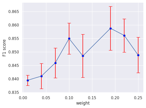
今回の試行では、平均値(青い点)はデフォルトの0.25よりも0.20付近が良い結果になりました。一方で誤差範囲(赤線)が広いことやランダムシード値の影響も考慮すると、試行回数次第で傾向が変わる可能性があります。weight配分はデフォルトのまま使用しても問題なさそうです。
また、0.01付近は誤差範囲が狭いにもかかわらず精度が低いため、Instance-wise contrasting は表現学習に重要なタスクだと分かりました。

---

最後まで読んでいただき、ありがとうございました！
論文紹介は初めての試みであったため、至らない点あればコメントいただけると嬉しいです。
本記事が皆さんの一助になれば幸いです。

Reference

• T-Rep: Representation Learning for Time Series using Time-Embeddings
  • arxiv
  • Github
• Time2Vec
• TS2Vec
• Time Series Classification Website