ggplot2は、通常自動的に色を決めてプロットするが、
scale_color_manualを使えば、ユーザーが指定した通りの色でプロットすることができる。
例えば、以下のような5色でプロットしたいとする。
# パッケージロード
library("ggplot2")

# 色指定関数
ggdefault_cols <- function(n){
    hcl(h=seq(15, 375-360/n, length=n)%%360, c=100, l=65)
}

# 独自に色を指定
# 赤、黄色、緑、青、紫になる
mycolor <- ggdefault_cols(5)
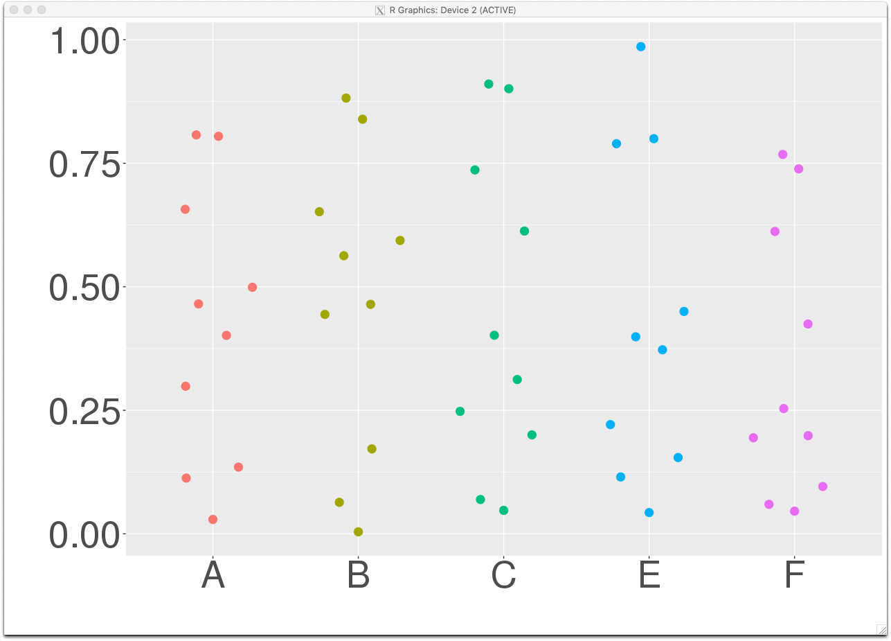
この色を使って、以下のような5つの手法のスコアの分布を、ビースウォームでプロットしてみる。
# テストデータ1(欠損値なし)
input1 = rbind(
	data.frame(Method="A", Score=runif(10)),
	data.frame(Method="B", Score=runif(10)),
	data.frame(Method="C", Score=runif(10)),
	data.frame(Method="E", Score=runif(10)),
	data.frame(Method="F", Score=runif(10))
)

# テストデータ1をまずプロット
g1 <- ggplot(input1, aes(x=Method, y=Score, color=Method))
g1 <- g1 + geom_quasirandom(dodge.width = 0.7, cex=4)
g1 <- g1 + ylim(0, ymax)
g1 <- g1 + ylab("") + xlab("")
g1 <- g1 + theme(text = element_text(size=50))
g1 <- g1 + theme(legend.position = 'none') + scale_color_manual(values = mycolor)
# 赤、黄色、緑、青、紫で出力される
g1
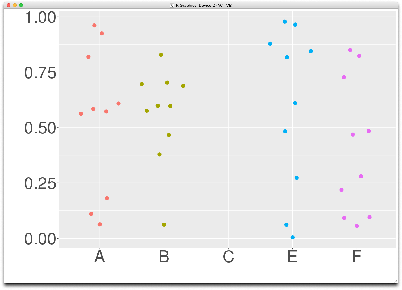
次に、似たようなデータだが、Cのスコアが何らかの理由により、得られなかったデータで同様にプロットする。
# テストデータ2(Cがまるまる欠損している)
input2 = rbind(
	data.frame(Method="A", Score=runif(10)),
	data.frame(Method="B", Score=runif(10)),
	data.frame(Method="C", Score=rep(NA, 10)),
	data.frame(Method="E", Score=runif(10)),
	data.frame(Method="F", Score=runif(10))
)

g2 <- ggplot(input2, aes(x=Method, y=Score, color=Method))
g2 <- g2 + geom_quasirandom(dodge.width = 0.7, cex=4)
g2 <- g2 + ylim(0, ymax)
g2 <- g2 + ylab("") + xlab("")
g2 <- g2 + theme(text = element_text(size=50))
g2 <- g2 + theme(legend.position = 'none') + scale_color_manual(values = mycolor)
g2
この場合、Cが欠損していることにより、Cに対応する緑はCでは使われず、D、Eに緑、青が指定され最後の紫は使われない。
つまり、欠損したC以降の色が全てずれてしまう。
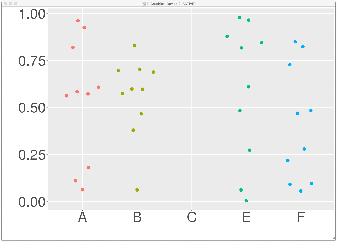
これは、scale_color_manualにdrop=FALSEというオプションを指定すると解決される。
g2_2 <- ggplot(input2, aes(x=Method, y=Score, color=Method))
g2_2 <- g2_2 + geom_quasirandom(dodge.width = 0.7, cex=4)
g2_2 <- g2_2 + ylim(0, ymax)
g2_2 <- g2_2 + ylab("") + xlab("")
g2_2 <- g2_2 + theme(text = element_text(size=50))
g2_2 <- g2_2 + theme(legend.position = 'none') + scale_color_manual(values = mycolor, drop=FALSE)
g2_2