目的
ランダムフォレスト(RF:random forest)は頻繁に使われる機械学習手法です。RFモデルは特徴量の重要度を確認できるので、特徴量の解釈にも使えます。
一方で、機械学習では一般に多重共線性が問題とされ、0.7ほどを目安に前処理で除くことが推奨されています。共線性の除去には、ドメイン知識の併用が望まれますが、膨大な場合にはとりあえず片方を消してしまうことが多く、その判断や基準は初学者には難しいです。
今回は、RFモデルであれば、実際に共線性がどれぐらいからどのような影響を与えるか検証してみました。
手法
サンプルデータセットを使ってRFモデルを作成
特徴量重要度の高かったものに対して意図的に相関の高い列を付加
予測精度と、特徴量の重要度スコアに与える影響を分析
基本パッケージ
今回は宗教上の理由でRのtidyverse系統を使います。
library(tidyverse)
library(tidymodels)
他に使うパッケージは以下で個別に使い、基本的にパッケージ名::の形で呼び出すようにしています。
データ準備
Breast Cancer Wisconsin (Diagnostic) Data Setの一部を使用
これは、良性腫瘍と悪性腫瘍のがん細胞の核の形の特徴量のデータです。
- 1列目に検体のID
- 2列目に良性腫瘍か悪性腫瘍かのラベル("B" = 良性腫瘍,"M" = 悪性腫瘍)。今回の目的変数
- 3列目以降に特徴量が格納。10種類の特徴量について平均値,標準誤差,最大値が順番に格納されていて計30列の項目
以下ではこのデータから10種類の特徴量の平均値のみを取りだして使います。
df_raw <- read_csv("https://archive.ics.uci.edu/ml/machine-learning-databases/breast-cancer-wisconsin/wdbc.data",
         col_names = c("ID", "Diagnosis", "Radius", "Texture", "Perimeter", "Area", "Smoothness",
           "Compactness", "Concavity", "Concave_points", "Symmetry", "Fractal_dimension")) |>
  select(ID:Fractal_dimension) |>
  mutate(ID = as.character(ID))
df_raw
# A tibble: 569 × 12
   ID       Diagnosis Radius Texture Perimeter  Area Smoothness Compactness Concavity Concave_points Symmetry Fractal_dimension
   <chr>    <chr>      <dbl>   <dbl>     <dbl> <dbl>      <dbl>       <dbl>     <dbl>          <dbl>    <dbl>             <dbl>
 1 842302   M           18.0    10.4     123.  1001      0.118       0.278     0.300          0.147     0.242            0.0787
 2 842517   M           20.6    17.8     133.  1326      0.0847      0.0786    0.0869         0.0702    0.181            0.0567
 3 84300903 M           19.7    21.2     130   1203      0.110       0.160     0.197          0.128     0.207            0.0600
 4 84348301 M           11.4    20.4      77.6  386.     0.142       0.284     0.241          0.105     0.260            0.0974
 5 84358402 M           20.3    14.3     135.  1297      0.100       0.133     0.198          0.104     0.181            0.0588
 6 843786   M           12.4    15.7      82.6  477.     0.128       0.17      0.158          0.0809    0.209            0.0761
 7 844359   M           18.2    20.0     120.  1040      0.0946      0.109     0.113          0.074     0.179            0.0574
 8 84458202 M           13.7    20.8      90.2  578.     0.119       0.164     0.0937         0.0598    0.220            0.0745
 9 844981   M           13      21.8      87.5  520.     0.127       0.193     0.186          0.0935    0.235            0.0739
10 84501001 M           12.5    24.0      84.0  476.     0.119       0.240     0.227          0.0854    0.203            0.0824
実行
前処理
相関分析
df_raw |> select(!where(is.character)) |> cor() |>
  corrplot::corrplot(method="shade", shade.col=NA,
                     tl.col="black",
                     col = corrplot::COL2('PRGn'), addCoef.col = 'grey60')
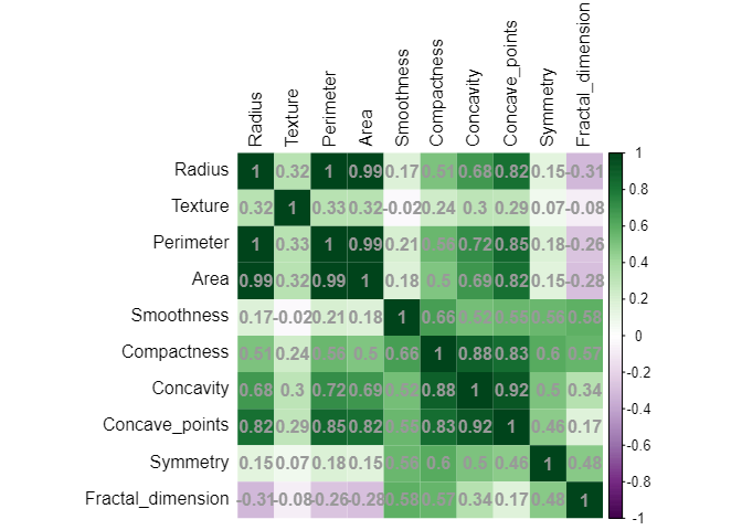
相関が高いものを除きます。今回は片側を無慈悲に捨てましょう。
# カスタム関数を作成して多重共線性を検出し、変数を除去する
detect_and_remove_multicollinearity <- function(data, threshold) {
  cor_matrix <- cor(data)  # 相関行列を計算
  n <- ncol(cor_matrix)
  correlated_vars <- character(0)

  for (i in 1:(n - 1)) {
    for (j in (i + 1):n) {
      if (abs(cor_matrix[i, j]) > threshold) {
        # 相関係数がしきい値を超える場合、変数名をリストに追加
        correlated_vars <- c(correlated_vars, colnames(data)[i])
      }
    }
  }

  # 多重共線性が高い変数を除去
  data_reduced <- data[, -which(colnames(data) %in% correlated_vars)]

  return(data_reduced)
}

df_rm <- df_raw |> select(!where(is.character)) |>
  detect_and_remove_multicollinearity(threshold = 0.7) |>
  bind_cols(df_raw |> select(where(is.character))) |>
  select(ID,Diagnosis,everything())


df_rm |> select(!where(is.character)) |> cor() |>
  corrplot::corrplot(method="shade", shade.col=NA,
                     tl.col="black",
                     col = corrplot::COL2('PRGn'), addCoef.col = 'grey60')
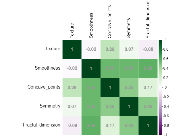
共線性を除けた
df_rm
# A tibble: 569 × 7
   ID       Diagnosis Texture Smoothness Concave_points Symmetry Fractal_dimension
   <chr>    <chr>       <dbl>      <dbl>          <dbl>    <dbl>             <dbl>
 1 842302   M            10.4     0.118          0.147     0.242            0.0787
 2 842517   M            17.8     0.0847         0.0702    0.181            0.0567
 3 84300903 M            21.2     0.110          0.128     0.207            0.0600
 4 84348301 M            20.4     0.142          0.105     0.260            0.0974
 5 84358402 M            14.3     0.100          0.104     0.181            0.0588
 6 843786   M            15.7     0.128          0.0809    0.209            0.0761
 7 844359   M            20.0     0.0946         0.074     0.179            0.0574
 8 84458202 M            20.8     0.119          0.0598    0.220            0.0745
 9 844981   M            21.8     0.127          0.0935    0.235            0.0739
10 84501001 M            24.0     0.119          0.0854    0.203            0.0824
現状の重要度の確認と、モデル設定
相関の高い特徴量を与える指標を探すために、現状のデータでの確認と、今回のデータに適合させるモデル・ハイパラ設定を行います。
個別前処理
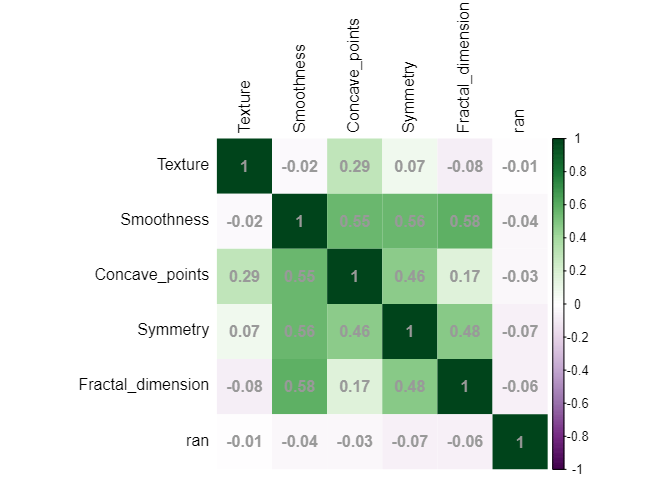
乱数の列を加えます。
今後のダミー特徴量を追加したときの列数を揃えるためです。
set.seed(123)
df_random <- df_rm |> mutate(ran = rnorm(569, mean =0, sd =1))

df_random |> select(!where(is.character)) |> cor() |>
  corrplot::corrplot(method="shade", shade.col=NA,
                     tl.col="black",
                     col = corrplot::COL2('PRGn'), addCoef.col = 'grey60')
モデルの設定
以下は一般的なtidymodelsの話です。
本筋ではないので、あまり詳しくはふれません。
テストデータとトレーニングデータに分割
split_df <- initial_split(df_random, strata = Diagnosis, prop=0.8)
train_data <- training(split_df)
test_data <- testing(split_df)
バリデーションデータの作成
cv_data <- train_data |> vfold_cv(strata = Diagnosis,v=10)
前処理
rec_base <- recipe(Diagnosis ~ ., data = train_data) |>
  step_rm(ID) |>
  step_normalize(all_numeric(),-all_outcomes())
モデル指定
ml_rf <- rand_forest(
  mtry = tune(),
  trees = 500,
  min_n = tune()
) |>
  set_mode("classification") |> # 分類モデルを指定
  set_engine("ranger",importance = "impurity") # importanceを出すように指定
ワークフローの作成
wf_base <- workflow() |>
 add_recipe(rec_base) |>
 add_model(ml_rf)
ハイパラ探索
# レンジの指定。適時調整
param_rf <- list(min_n(range=c(2,10)),
                 mtry(range = c(2,6))
                 ) |>
  dials::parameters()

# ベイズ最適化
res_bayes <- wf_base |>
  tune_bayes(resamples = cv_data,
             param_info = param_rf,
             initial = 5,
             iter = 20,
             metrics = yardstick::metric_set(accuracy,roc_auc))
探索結果
res_bayes |> autoplot()
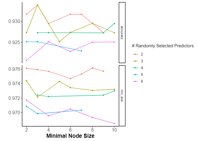
mtryが大きいと良くなさそう。もう少し探索してもいいが、今回はこれでよし。
res_bayes |> show_best(metric = "accuracy")
# A tibble: 5 × 9
  min_n  mtry .metric  .estimator  mean     n std_err .config              .iter
  <int> <int> <chr>    <chr>      <dbl> <int>   <dbl> <chr>                <int>
1     4     2 accuracy binary     0.934    10  0.0119 Iter4                    4
2     8     2 accuracy binary     0.934    10  0.0132 Iter7                    7
3     4     3 accuracy binary     0.932    10  0.0134 Preprocessor1_Model1     0
4     7     2 accuracy binary     0.932    10  0.0125 Preprocessor1_Model4     0
5     2     2 accuracy binary     0.932    10  0.0138 Iter2                    2
モデルの設定と更新
# accuracyが一番いいのを取ってくる
best_param <-
  res_bayes |>
  select_best("accuracy")

wf_best <- wf_base |> finalize_workflow(best_param)
適用
res_all <- wf_best |>
   tune::last_fit(split_df)
テストデータでの当てはまり
collect_metrics(res_all)
# A tibble: 2 × 4
  .metric  .estimator .estimate .config
  <chr>    <chr>          <dbl> <chr>
1 accuracy binary         0.948 Preprocessor1_Model1
2 roc_auc  binary         0.974 Preprocessor1_Model1
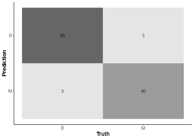
res_all |> collect_predictions() |> conf_mat(Diagnosis,.pred_class) |> autoplot(type="heatmap")
res_all |> collect_predictions() |> roc_curve(Diagnosis,.pred_B) |> autoplot()
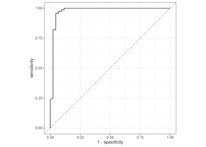
これが目安になります。このデータに対して、ランダムフォレストモデルで予測はできそうです。
重要度
res_all |> extract_fit_parsnip() |> vip::vip()
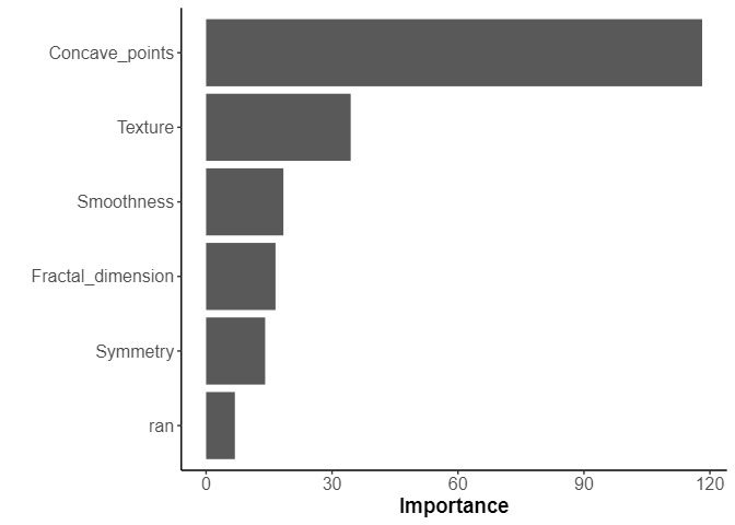
これが欲しかったものです。
「Concave_point=輪郭の凹部の数=輪郭の凸凹度合い」がとても強いので、この子に相関性の高いダミーデータを当てて様子をみてみます。
ダミーデータの生成
現在の特徴量に乱数を加えて相関の高い列を加える
add_randf <- function(sd_param) {
  set.seed(123)
  random_var <- rnorm(569, mean =0, sd =sd_param)
  df_random <- df_rm |> mutate(ran = Concave_points + random_var)
  return(df_random)
}

df_test_ran <- add_randf(0.01)
cor_val <- cor(df_test_ran$Concave_points,df_test_ran$ran)
df_test_ran |>
  ggplot(aes(x=Concave_points,y=ran)) +
  geom_point() +
  ggtitle(label = str_glue("cor = {round(cor_val, 3)}"))
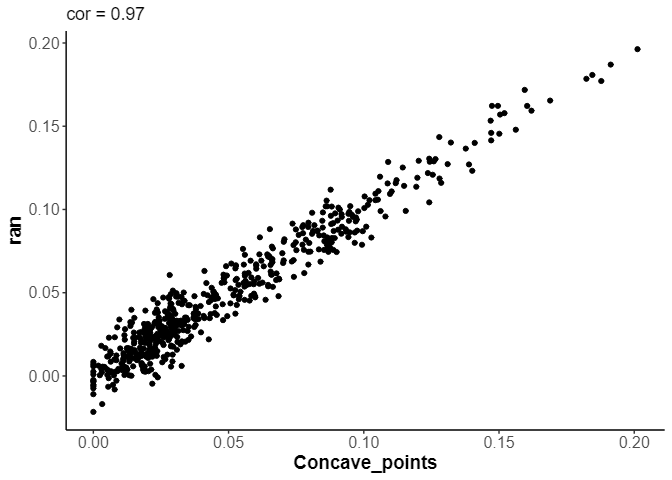
こんな感じに相関の高いダミー特徴量を生成できました。
sdを変えることで相関の高さを変え、
複数のデータに対して、先ほど作成したモデルを適用させて学習させていきます。
fit_data <- tibble(sd_val = seq(0,0.1,by=0.005)) |>
  mutate(base_data = map(sd_val,add_randf),
         cor_val = map_dbl(base_data,~ cor(.$Concave_points,.$ran)),
         fittted = map(base_data,
                       ~ wf_best |> tune::last_fit(initial_split(., strata = Diagnosis, prop=0.8))))
モデルから結果を抽出
- accuracy
- importance
cal_data <- fit_data |>
  mutate(accuracy = map_dbl(fittted,
                        ~ . |> collect_metrics() %>%
                          filter(.metric == "accuracy") %>%
                          pull(.estimate)),
         importance_df = map(fittted,
                             ~ . |> extract_fit_engine() |>
                               importance() |> as_tibble_row() |>
                               pivot_longer(cols=everything())))
cal_data
# A tibble: 21 × 6
   sd_val base_data          cor_val fittted   accuracy importance_df
    <dbl> <list>               <dbl> <list>       <dbl> <list>
 1  0     <tibble [569 × 8]>   1     <rsmp[+]>    0.957 <tibble [6 × 2]>
 2  0.005 <tibble [569 × 8]>   0.992 <rsmp[+]>    0.922 <tibble [6 × 2]>
 3  0.01  <tibble [569 × 8]>   0.970 <rsmp[+]>    0.922 <tibble [6 × 2]>
 4  0.015 <tibble [569 × 8]>   0.936 <rsmp[+]>    0.913 <tibble [6 × 2]>
 5  0.02  <tibble [569 × 8]>   0.893 <rsmp[+]>    0.939 <tibble [6 × 2]>
 6  0.025 <tibble [569 × 8]>   0.845 <rsmp[+]>    0.930 <tibble [6 × 2]>
 7  0.03  <tibble [569 × 8]>   0.795 <rsmp[+]>    0.939 <tibble [6 × 2]>
 8  0.035 <tibble [569 × 8]>   0.746 <rsmp[+]>    0.948 <tibble [6 × 2]>
 9  0.04  <tibble [569 × 8]>   0.699 <rsmp[+]>    0.930 <tibble [6 × 2]>
10  0.045 <tibble [569 × 8]>   0.654 <rsmp[+]>    0.939 <tibble [6 × 2]>
結果
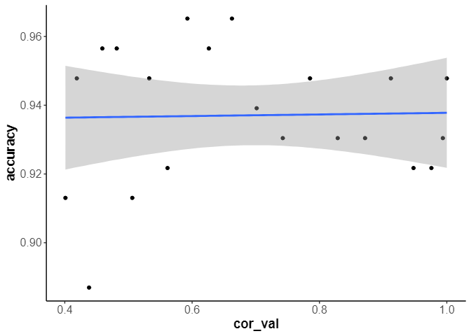
accuracyの傾向
cal_data |>
  ggplot(aes(x=cor_val,y=accuracy)) +
  geom_point() +
  geom_smooth(method = 'glm',formula = 'y ~ x')
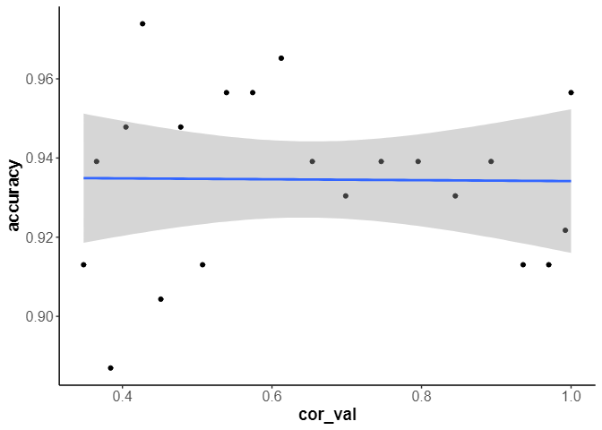
精度には影響がないようです。
特徴量重要度の傾向
まず、対象にしたConcave_pointの重要度の変化をみます。
cal_data |>
  unnest(importance_df) |>
  filter(name=="Concave_points") |>
  ggplot(aes(x=cor_val,y=value)) +
  geom_point() +
  geom_smooth(method = 'loess',formula = 'y ~ x')
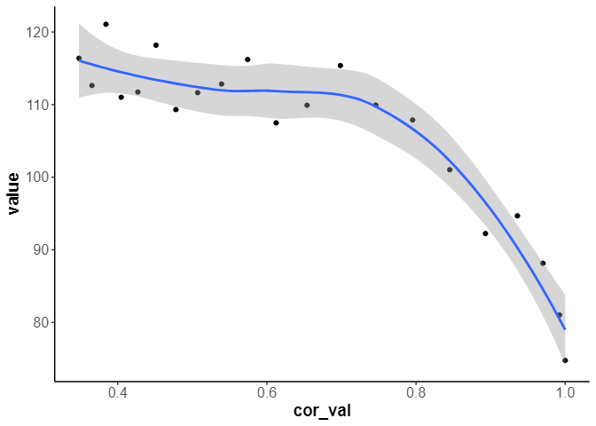
0.7より相関が高いものがあると、特徴量重要度は低下する様子が見えました。
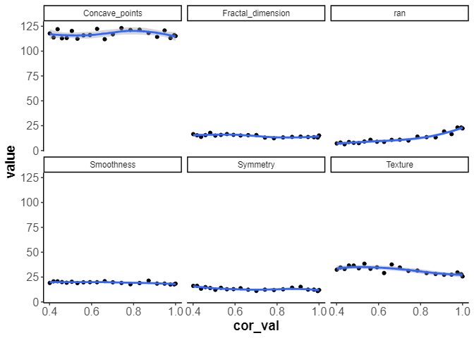
他の指標はどうでしょうか。
cal_data |>
  unnest(importance_df) |>
  ggplot(aes(x=cor_val,y=value)) +
  geom_point() +
  geom_smooth(method = 'loess',formula = 'y ~ x') +
  facet_wrap(vars(name))
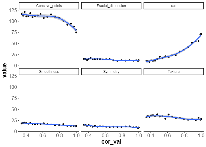
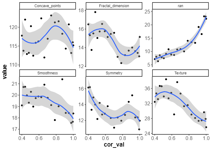
スケールを揃えないものも確認
cal_data |>
  unnest(importance_df) |>
  ggplot(aes(x=cor_val,y=value)) +
  geom_point() +
  geom_smooth(method = 'loess',formula = 'y ~ x') +
  facet_wrap(vars(name), scales = "free_y")
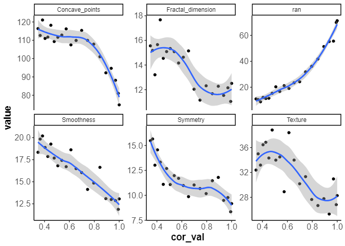
他の指標も負の影響を受けるが、その変化は微小です。
乱数の指標は相関が高くなればなるほど、重要度は増えていくのは妥当です。
結論・考察
ランダムフォレストに共線性は、精度にはほぼ影響を与えませんでした。一方で、特徴量の重要度には0.7を目安に共線性を除去しなければ影響を与え、特徴量を理解する場合には注意が必要です。
代役(相関が高い指標)が他にいても、劇自体は問題なくなりたつので精度には影響はないですが、人気(特徴量重要度)が分散して特徴量としては共倒れするような現象が起きているようです。
おまけ
序列2位の"Texture"に対して行うとどうなるのでしょうか。
Accuracy
特徴量重要度
やはり、精度には影響はないです。
しかし、対象となった指標の重要度は0.7あたりを基準に下がるようすがみられます。Concave_pointsが影響を受けないので、純粋に指標が増えたら下がるとかではないのが確認できました。