用途
推しポイント
- 機械学習もtidyに行いたい人向け
- 色々なアルゴリズムを並列して実施できる
- パッケージごとに異なる変数を使っているのを統合可能
主なことはRユーザのためのtidymodels[実践]入門に書いてます。
ここでは使ってみたのを書いておきます。
コード
手法
みんな大好きirisで分類を実施
library(tidyverse)
library(tidymodels)

df_raw <- iris |> tibble()
実行
RFモデルで品種予測させてみる
バリデーション作成
10-foldのCVを行う strataで品種を指定してバリデーションの偏りをなくす
cv_data <- df_raw |> vfold_cv(strata = Species,v=10)
処理の確認
cv_data
## #  10-fold cross-validation using stratification
## # A tibble: 10 × 2
##    splits           id
##    <list>           <chr>
##  1 <split [135/15]> Fold01
##  2 <split [135/15]> Fold02
##  3 <split [135/15]> Fold03
##  4 <split [135/15]> Fold04
##  5 <split [135/15]> Fold05
##  6 <split [135/15]> Fold06
##  7 <split [135/15]> Fold07
##  8 <split [135/15]> Fold08
##  9 <split [135/15]> Fold09
## 10 <split [135/15]> Fold10
cv_data$splits[[1]] |> assessment()
## # A tibble: 15 × 5
##    Sepal.Length Sepal.Width Petal.Length Petal.Width Species
##           <dbl>       <dbl>        <dbl>       <dbl> <fct>
##  1          5.1         3.5          1.4         0.2 setosa
##  2          5.4         3.7          1.5         0.2 setosa
##  3          4.8         3            1.4         0.1 setosa
##  4          5.4         3.4          1.5         0.4 setosa
##  5          5.3         3.7          1.5         0.2 setosa
##  6          6.9         3.1          4.9         1.5 versicolor
##  7          5.7         2.8          4.5         1.3 versicolor
##  8          5.6         2.5          3.9         1.1 versicolor
##  9          6.7         3            5           1.7 versicolor
## 10          6.3         2.3          4.4         1.3 versicolor
## 11          6.3         3.3          6           2.5 virginica
## 12          6.9         3.2          5.7         2.3 virginica
## 13          6.4         2.8          5.6         2.2 virginica
## 14          6.3         2.8          5.1         1.5 virginica
## 15          6           3            4.8         1.8 virginica
前処理
何を予測させるかの指示と、正規化などの前処理をrecipeに指定
rec_base <- recipe(Species ~ ., data=df_raw) |> # ここではデータ全体を使って正規化する
  step_normalize(all_numeric(), -all_outcomes())
処理の確認
rec_base |> prep() |> bake(new_data = NULL)
## # A tibble: 150 × 5
##    Sepal.Length Sepal.Width Petal.Length Petal.Width Species
##           <dbl>       <dbl>        <dbl>       <dbl> <fct>
##  1       -0.898      1.02          -1.34       -1.31 setosa
##  2       -1.14      -0.132         -1.34       -1.31 setosa
##  3       -1.38       0.327         -1.39       -1.31 setosa
##  4       -1.50       0.0979        -1.28       -1.31 setosa
##  5       -1.02       1.25          -1.34       -1.31 setosa
##  6       -0.535      1.93          -1.17       -1.05 setosa
##  7       -1.50       0.786         -1.34       -1.18 setosa
##  8       -1.02       0.786         -1.28       -1.31 setosa
##  9       -1.74      -0.361         -1.34       -1.31 setosa
## 10       -1.14       0.0979        -1.28       -1.44 setosa
## # ℹ 140 more rows
モデル指定
ここではrangerパッケージを使ってRFを行う
mtryとmin_nは後でハイパラ探索するのでtune()とする。
ml_rf <- rand_forest(
  mtry = tune(),
  trees = 500,
  min_n = tune()
) |>
  set_mode("classification") |> # 分類モデルを指定
  set_engine("ranger",importance = "impurity") # importanceを出すように指定
ワークフロー
recipeをモデルの一連の解析を一度にできるようにワークフローを設定 無しでもできる。
wf_base <- workflow() |>
 add_recipe(rec_base) |>
 add_model(ml_rf)
ハイパラ探索
検証したいレンジを指定して実施
# レンジの指定。適時調整
param_rf <- list(min_n(range=c(1,5)),
                 mtry(range = c(1,4))
                 ) |>
  dials::parameters()

# グリッドサーチでの探索点を指定
set.seed(11)
grid_range <- param_rf |>
  dials::grid_random(size=10) # 今回はパラメータ探索幅が少ないので10個も多分出ない

# 探索実施
res_grid <- wf_base |>
  tune_grid(resamples = cv_data,
            grid = grid_range,
            # control = control_grid(save_pred = TRUE), # 予測値を残すか
            metrics = yardstick::metric_set(accuracy,roc_auc)) # 判定したいスコアを指定
パラメータ探索の結果
res_grid |> show_best(metric = "accuracy")
## # A tibble: 5 × 8
##    mtry min_n .metric  .estimator  mean     n std_err .config
##   <int> <int> <chr>    <chr>      <dbl> <int>   <dbl> <chr>
## 1     2     5 accuracy multiclass 0.967    10  0.0111 Preprocessor1_Model05
## 2     3     4 accuracy multiclass 0.967    10  0.0111 Preprocessor1_Model07
## 3     4     5 accuracy multiclass 0.967    10  0.0111 Preprocessor1_Model08
## 4     3     5 accuracy multiclass 0.967    10  0.0111 Preprocessor1_Model09
## 5     3     3 accuracy multiclass 0.96     10  0.0147 Preprocessor1_Model10
res_grid |> autoplot()

説明変数は3つがよさそう
モデル設定と更新
# 結果確認
res_grid |> collect_metrics()
## # A tibble: 20 × 8
##     mtry min_n .metric  .estimator  mean     n std_err .config
##    <int> <int> <chr>    <chr>      <dbl> <int>   <dbl> <chr>
##  1     1     2 accuracy multiclass 0.947    10 0.0133  Preprocessor1_Model01
##  2     1     2 roc_auc  hand_till  0.993    10 0.00358 Preprocessor1_Model01
##  3     3     2 accuracy multiclass 0.953    10 0.0174  Preprocessor1_Model02
##  4     3     2 roc_auc  hand_till  0.996    10 0.00285 Preprocessor1_Model02
##  5     3     1 accuracy multiclass 0.953    10 0.0174  Preprocessor1_Model03
##  6     3     1 roc_auc  hand_till  0.996    10 0.00285 Preprocessor1_Model03
##  7     1     1 accuracy multiclass 0.947    10 0.0133  Preprocessor1_Model04
##  8     1     1 roc_auc  hand_till  0.993    10 0.00358 Preprocessor1_Model04
##  9     2     5 accuracy multiclass 0.967    10 0.0111  Preprocessor1_Model05
## 10     2     5 roc_auc  hand_till  0.995    10 0.00295 Preprocessor1_Model05
## 11     1     4 accuracy multiclass 0.947    10 0.0133  Preprocessor1_Model06
## 12     1     4 roc_auc  hand_till  0.993    10 0.00358 Preprocessor1_Model06
## 13     3     4 accuracy multiclass 0.967    10 0.0111  Preprocessor1_Model07
## 14     3     4 roc_auc  hand_till  0.996    10 0.00285 Preprocessor1_Model07
## 15     4     5 accuracy multiclass 0.967    10 0.0111  Preprocessor1_Model08
## 16     4     5 roc_auc  hand_till  0.996    10 0.00285 Preprocessor1_Model08
## 17     3     5 accuracy multiclass 0.967    10 0.0111  Preprocessor1_Model09
## 18     3     5 roc_auc  hand_till  0.996    10 0.00285 Preprocessor1_Model09
## 19     3     3 accuracy multiclass 0.96     10 0.0147  Preprocessor1_Model10
## 20     3     3 roc_auc  hand_till  0.996    10 0.00285 Preprocessor1_Model10
# accuracyが一番いいのを取ってくる
best_param <-
  res_grid |>
  select_best("accuracy")

# いいハイパラでワークフローの更新
wf_best <- wf_base |>
  finalize_workflow(best_param)
適用
res_best <- wf_best |>
  fit_resamples(resamples = cv_data, control = control_resamples(save_pred = TRUE))

collect_metrics(res_best)
## # A tibble: 2 × 6
##   .metric  .estimator  mean     n std_err .config
##   <chr>    <chr>      <dbl> <int>   <dbl> <chr>
## 1 accuracy multiclass 0.967    10 0.0111  Preprocessor1_Model1
## 2 roc_auc  hand_till  0.995    10 0.00295 Preprocessor1_Model1
df_pred <- augment(res_best)
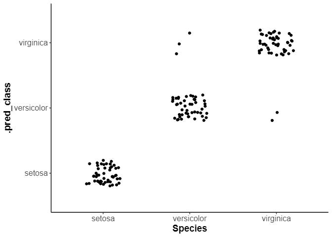
可視化
df_pred |>
  ggplot(aes(x=Species, y=.pred_class)) +
  geom_jitter(width = 0.2,height = 0.2)
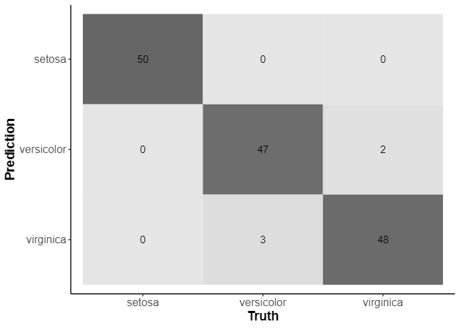
混同行列
res_best |> collect_predictions() |> conf_mat(Species,.pred_class) |> autoplot(type="heatmap")
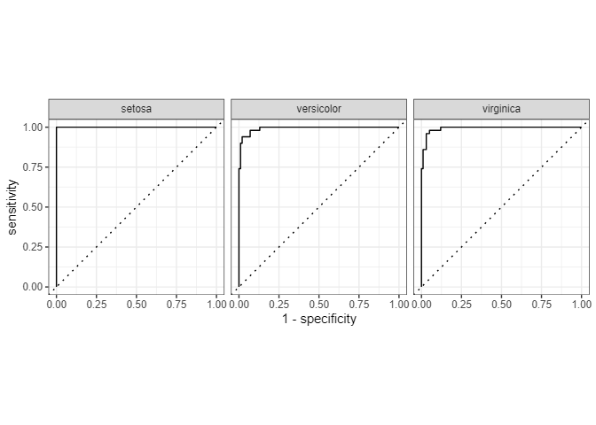
ROC_curve
res_best |> collect_predictions() |> roc_curve(Species, .pred_setosa:.pred_virginica) |> autoplot()
setosaは楽勝といういつもの流れ
重要度
各cvのモデルの重要度を取得
# CV
fit_eachcv <- function(split_data) {
  wf_best |> fit(analysis(split_data)) |>
    extract_fit_engine() |> importance() |> as.table()
}

cv_fit <- cv_data |> mutate(importance = map_dfr(splits, fit_eachcv)) |> pull(importance)
cv_fit |> as.matrix() |> t() |> as.data.frame() |>
  rownames_to_column() |>
  pivot_longer(cols = -rowname) |>
  ggplot(aes(x=reorder(rowname,value,FUN = mean),y=value)) +
  stat_summary(geom = "bar", fun=mean,position = "dodge") +
  stat_summary(fun.min = function(x) mean(x) - sd(x), fun.max = function(x) mean(x) + sd(x),geom = "errorbar",position = "dodge", width = 0.3, size = 1) +
  labs(x=NULL) +
  coord_flip()
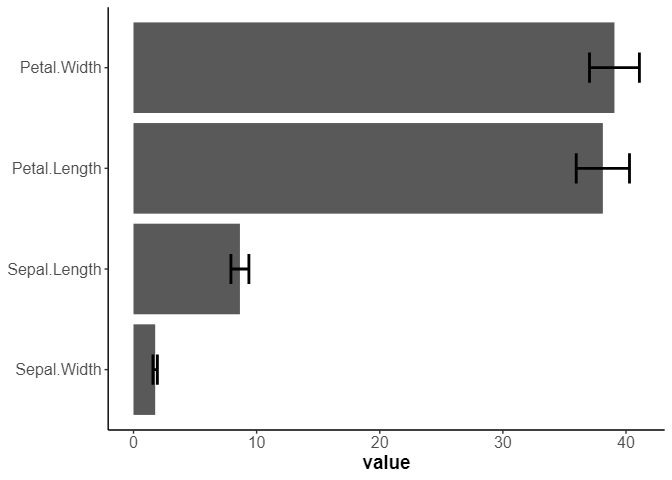
2強状態
三角図で確率を示す
(執筆時点ではggternがCRANから外れていたので、こちらを参考にした。戻っているのでggternを使った方が楽。)
色は正解ラベル
gg_tripred <- function(df_pred) {
  axis_lab <- c("pred_setosa","pred_versicolor","pred_virginica")


  # 軸目盛の位置を指定
  axis_vals <- seq(from = 0, to = 1, by = 0.1)
  # 枠線用の値を作成
  ternary_axis_df <- tibble::tibble(
    y_1_start = c(0.5, 0, 1),         # 始点のx軸の値
    y_2_start = c(0.5*sqrt(3), 0, 0), # 始点のy軸の値
    y_1_end = c(0, 1, 0.5),           # 終点のx軸の値
    y_2_end = c(0, 0, 0.5*sqrt(3)),   # 終点のy軸の値
    axis = c("x_1", "x_2", "x_3")     # 元の軸
  )
  # グリッド線用の値を作成
  ternary_grid_df <- tibble::tibble(
    y_1_start = c(
      0.5 * axis_vals,
      axis_vals,
      0.5 * axis_vals + 0.5
    ), # 始点のx軸の値
    y_2_start = c(
      sqrt(3) * 0.5 * axis_vals,
      rep(0, times = length(axis_vals)),
      sqrt(3) * 0.5 * (1 - axis_vals)
    ), # 始点のy軸の値
    y_1_end = c(
      axis_vals,
      0.5 * axis_vals + 0.5,
      0.5 * rev(axis_vals)
    ), # 終点のx軸の値
    y_2_end = c(
      rep(0, times = length(axis_vals)),
      sqrt(3) * 0.5 * (1 - axis_vals),
      sqrt(3) * 0.5 * rev(axis_vals)
    ), # 終点のy軸の値
    axis = c("x_1", "x_2", "x_3") |>
      rep(each = length(axis_vals)) # 元の軸
  )
  # 軸ラベル用の値を作成
  ternary_axislabel_df <- tibble::tibble(
    y_1 = c(0.25, 0.5, 0.75),               # x軸の値
    y_2 = c(0.25*sqrt(3), 0, 0.25*sqrt(3)), # y軸の値
    label = axis_lab,      # 軸ラベル
    h = c(1.5, 0.5, -0.5),  # 水平方向の調整用の値
    v = c(0.5, 2.5, 0.5), # 垂直方向の調整用の値
    axis = c("x_1", "x_2", "x_3") # 元の軸
  )
  # 軸目盛ラベル用の値を作成
  ternary_ticklabel_df <- tibble::tibble(
    y_1 = c(
      0.5 * axis_vals,
      axis_vals,
      0.5 * axis_vals + 0.5
    ), # x軸の値
    y_2 = c(
      sqrt(3) * 0.5 * axis_vals,
      rep(0, times = length(axis_vals)),
      sqrt(3) * 0.5 * (1 - axis_vals)
    ), # y軸の値
    label = c(
      rev(axis_vals),
      axis_vals,
      rev(axis_vals)
    ), # 軸目盛ラベル
    h = c(
      rep(1.5, times = length(axis_vals)),
      rep(1.5, times = length(axis_vals)),
      rep(-0.5, times = length(axis_vals))
    ), # 水平方向の調整用の値
    v = c(
      rep(0.5, times = length(axis_vals)),
      rep(0.5, times = length(axis_vals)),
      rep(0.5, times = length(axis_vals))
    ), # 垂直方向の調整用の値
    angle = c(
      rep(-60, times = length(axis_vals)),
      rep(60, times = length(axis_vals)),
      rep(0, times = length(axis_vals))
    ), # ラベルの表示角度
    axis = c("x_1", "x_2", "x_3") |>
      rep(each = length(axis_vals)) # 元の軸
  )

  # 三角座標に変換して格納
  data_df <- df_pred |>
    mutate(
      x_1 = .pred_setosa, # 元のx軸の値
      x_2 = .pred_versicolor, # 元のy軸の値
      x_3 = .pred_virginica, # 元のz軸の値
      y_1 = x_2 + 0.5 * x_3,     # 変換後のx軸の値
      y_2 = sqrt(3) * 0.5 * x_3, # 変換後のy軸の値
      label = str_c("(", round(x_1, 2), ", ", round(x_2, 2), ", ", round(x_3, 2), ")")
    )

  # 三角図の各軸を可視化
  ggplot() +
    geom_segment(data = ternary_axis_df,
                 mapping = aes(x = y_1_start, y = y_2_start, xend = y_1_end, yend = y_2_end),
                 color = "gray50") + # 三角図の枠線
    geom_segment(data = ternary_grid_df,
                 mapping = aes(x = y_1_start, y = y_2_start, xend = y_1_end, yend = y_2_end),
                 linetype = "dashed") + # 三角図のグリッド線
    geom_text(data = ternary_ticklabel_df,
              mapping = aes(x = y_1, y = y_2, label = label, hjust = h, vjust = v, angle = angle)) + # 三角図の軸目盛ラベル
    geom_text(data = ternary_axislabel_df,
              mapping = aes(x = y_1, y = y_2, label = label, hjust = h, vjust = v),
              parse = TRUE, size = 6) + # 三角図の軸ラベル
    geom_point(data = data_df,
               mapping = aes(x = y_1, y = y_2, color=Species),
               size = 3) + # 観測データ
    scale_x_continuous(breaks = c(0, 0.5, 1), labels = NULL) + # x軸
    scale_y_continuous(breaks = c(0, 0.25*sqrt(3), 0.5*sqrt(3)), labels = NULL) + # y軸
    scale_color_brewer(palette = "Set2") +
    coord_fixed(ratio = 1, clip = "off") + # アスペクト比
    theme(
      axis.ticks = element_blank(), # 目盛の指示線
      panel.grid.minor = element_blank(), # 補助目盛のグリッド線
      legend.position = c(0.8,0.8) # 凡例の位置
    ) + # 図の体裁
    labs(x = "", y = "") +
    theme(
      axis.line = element_blank()
    )
}

gg_tripred(df_pred = df_pred)
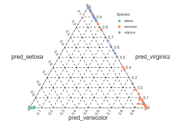
setosaは楽勝 自信もって間違えている点もあるので、かなり難しいか実データなら誤ラベルも考えられる
備考
最初に話した本が一番です。
またここで行っているCVはモデルの汎化性能を評価する交差検証であり、ハイパラ探索は一番当てられたものを釣ってきています。
つまり、ハイパラ探索をやらずに出しているものに比べたら予測がfitするので、モデルの信頼度が高くできる一方で、未知なものへの予測の保証はあまりありません。大切な特徴量を分析する目的で利用しています。