What is ARIMA?
ARIMA is short for Autoregressive Integrated Moving Average. An ARIMA model takes in three parameters:
- p : the number of time lags
- d : the degree of differencing
- q : the order of the moving average
It is usually made fit to a historical time series data and used to forecast future points in that series. Common applications of an ARIMA model may involve product demand predictions, price predictions, visitor estimations, or any of the above but with a seasonal trend.
Source Code
https://github.com/andy971022/SP500-ARIMA
When to Use Arima?
- When you have a time series data.
- When your time series data is stationary with respect to a certain order of differencing.
- When you want to predict the near future.
What Do You Mean by Stationary?
- Definition
- In Short: Your data does not show a time-depending trend.
Examples
The following images will show up again in our tutorial, but we'll use them to explain what a stationary process is. The first image down below is S&P500 ETF's(SPY) historical stock prices, and the second image is the second differentiation of that stock price from August 2019 to November 2019.
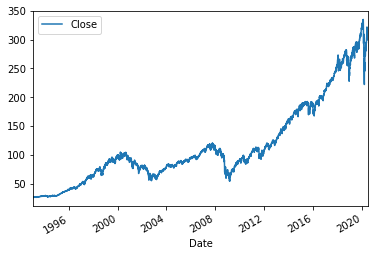
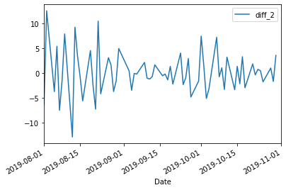
The process in the first image is not stationary because it has an obviously up-going trend correlating with time. The second image, however, shows a stationary process because the data points revolve around a constant value, meaning that they do not vary and correlate with time.
Steps to Creating an ARIMA Model
- Collect a set of time series data.
- Obtain the parameter d : do an ADF(augmented Dickey–Fuller test) test on the dataset with respect to various orders of differencing to obtain a stationary process.
- Obtain the parameter p : do an Autocorrelation test on the dataset with respect to the selected order d.
- Obtain the parameter q : do a Partial Autocorrelation test on the dataset with respect to the selected order d.
- Create the ARIMA(p,d,q) model with the deduced parameters.
- Fit and forecast.
Step 1
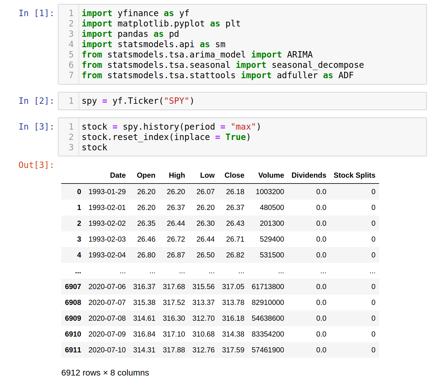
We'll get the historical closing stock prices for S&P500 from yfinance and predict the stock prices for November 2019.
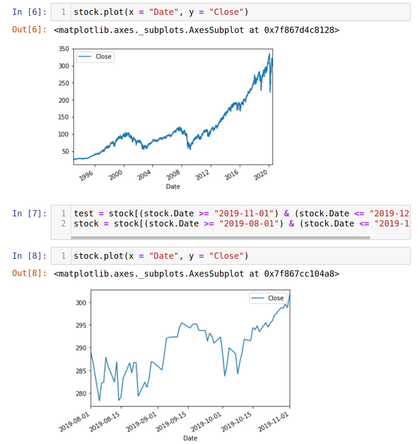
We plotted the graphs and saw that the stock prices are far from being stationary.
So, let's cherry-pick just the data three months prior to our target of prediction.
Step 2
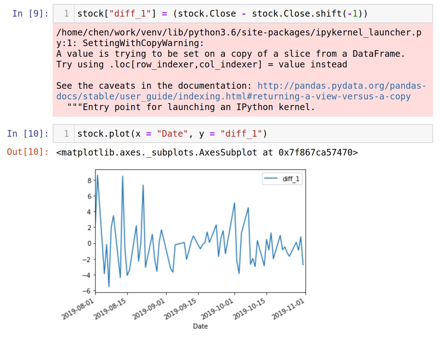
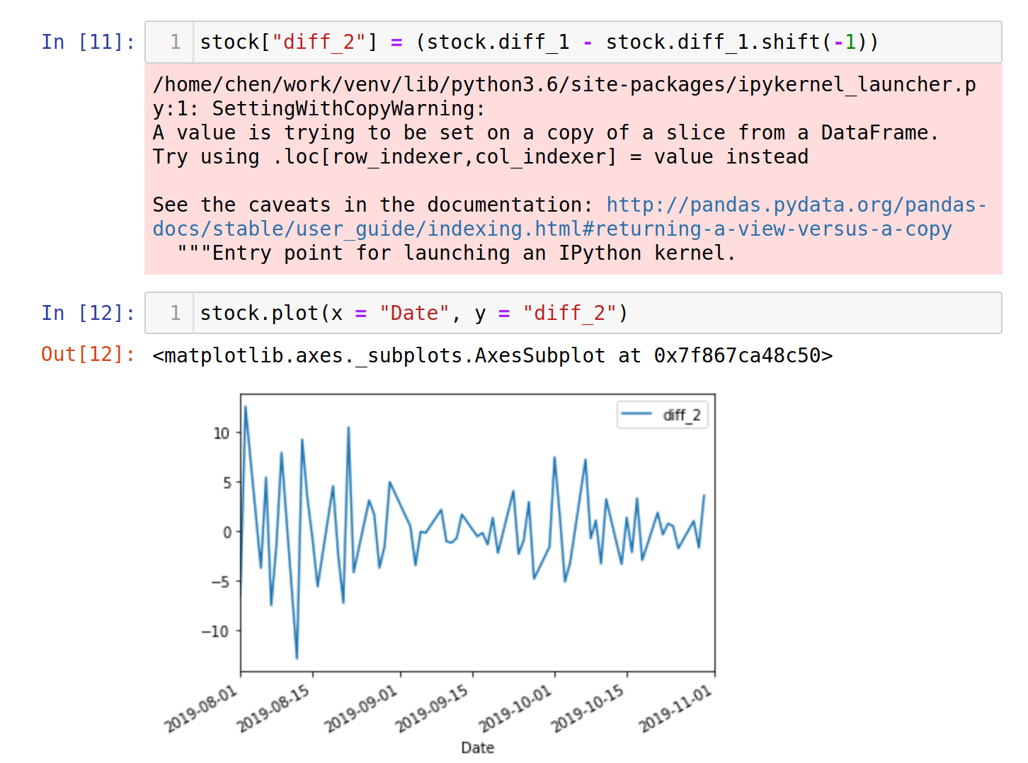
We'll create the first and second differences and compute the ADF tests following on.
The p-value of the first differentiation, -8.17674265403581, is less than -2.8853397507076006, the 5% alpha value, and even less than the 1% alpha value. That is, we can reject the null hypothesis and state that the data is stationary.
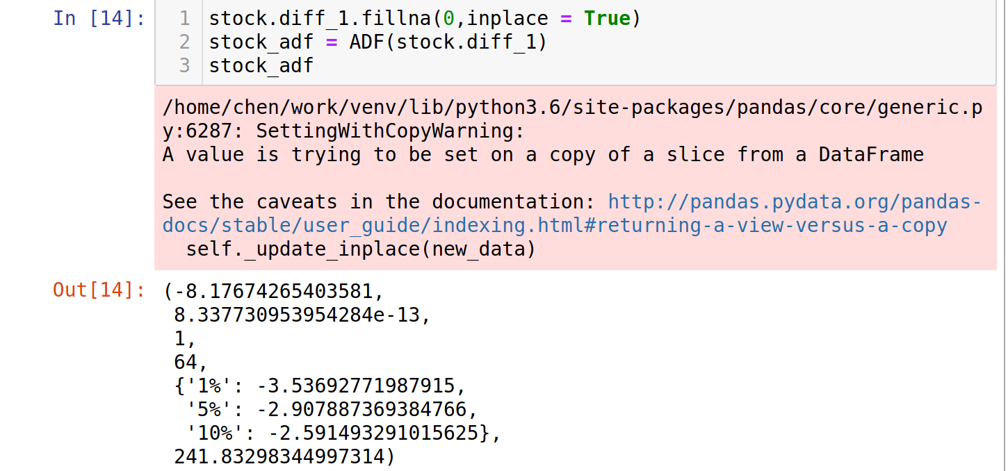
We see that the first difference is well enough for the ARIMA model. Therefore, we'll set the parameter d to 1.
Step 3
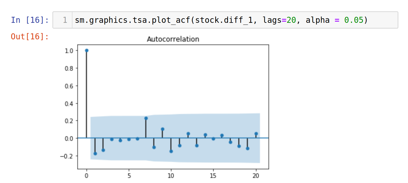
We have computed the autocorrelation test, and the result shows that 1 is a suitable value for p. Why? Because we need to truncate the first lag in order to have the rest of the autocorrelations fall within the 95% confidence interval, represented by the blue shades.
Step 4
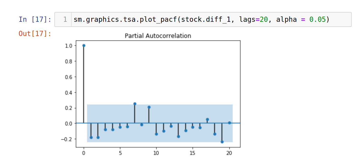
With similar reasons mentioned in Step 3, q is selected as one.
Step 5

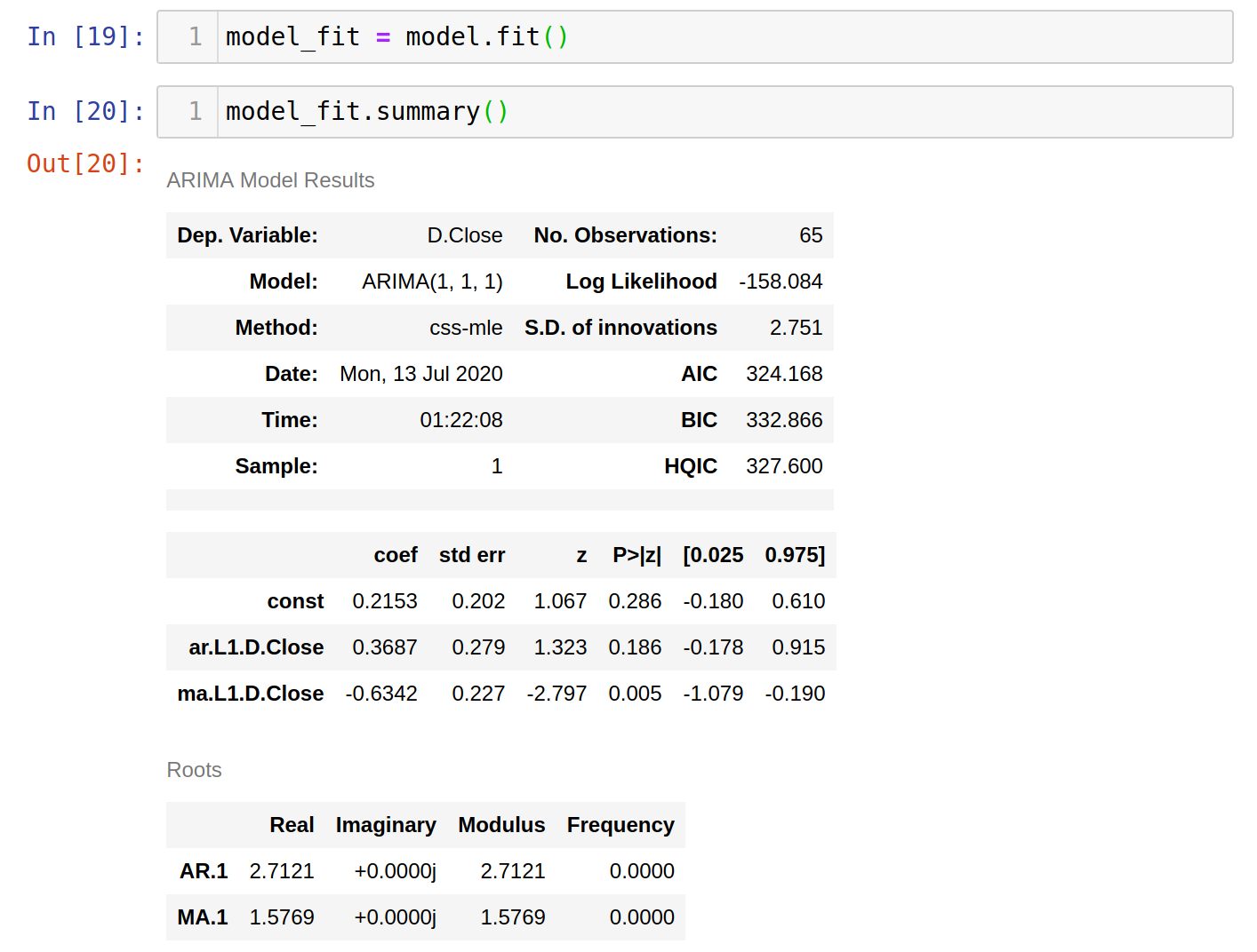
Now we have deduced an ARIMA(1,1,1) model and will fit the closing stock prices into the model. Be careful not to throw in the first difference of the stock price into the model.
Step 6
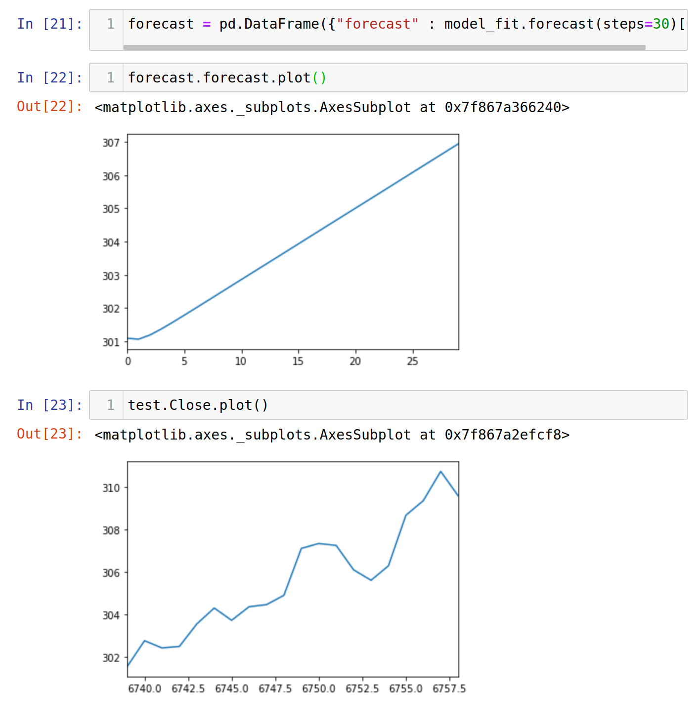
We have now fed data three months prior to our prediction into the model. The second last image is our prediction while the last one is the actual data. We see that our crude model can still be able to predict an accurate trend.