この記事では、PRML第5章で述べられている、全結合ニューラルネットワークによる多クラス分類器を実装します。
対応するjupyter notebookは筆者のgithubリポジトリにあります。連載の方針や、PRMLの他のアルゴリズムについては、連載のまとめページをご覧ください。
PRMLの本に載っている理論のおさらいをし、数式をコードに翻訳して、最後に実際に動かした結果を見ることにします。
1 理論のおさらい
この節では、PRMLに書かれている理論のおさらいをします。ただし、PRMLでの誤差逆伝播法の説明は記号の定義がやや雑に感じられた1ため、このノートではなるべく誤解のない記法を用いることにします。その分添え字が増えてしまっていますが、ご容赦を。。。
1.1 設定
このノートでは多クラス分類問題を解くニューラルネットワークを実装しますが、理論パートではなるべく一般的な書き方をしたいと思います2。
- $N \in \mathbb{N}$をデータの個数とします。
- $d \in \mathbb{N}$を入力の次元とします。
- $x_0, x_1, \dots , x_{N-1} \in \mathbb{R}^d$を入力データとします。
- 回帰問題については、target dataを$t_0, t_1, \dots, t_{N-1} \in \mathbb{R}$とします。
- 2クラス分類については、target dataを$t_0, t_1, \dots, t_{N-1} \in { 0, 1 }$とします。
- 多クラス分類問題については、$\mathcal{C} = \left\{ 0, 1, \dots, C-1 \right\}$をあり得るクラスラベルの集合、$t_0, t_1, \dots, t_{N-1} \in \left\{0,1\right\}^{C}$をtarget dataの1-of-$C$符号化とします(i.e., $n$番目のデータのラベルが$c$であれば、$t_n$は「$c$番目の要素が1、そのほかの要素が0のベクトル」となります。
1.2 モデル:ニューラルネットの表現
ここでは、$L$層の全結合フィードフォワードニューラルネットワークを考えることにします(下図参照。)。なお、「$L$層のニューラルネットワーク」は、ここでは$(L-1)$層の隠れ層を持つニューラルネットワークを意味するものとします。
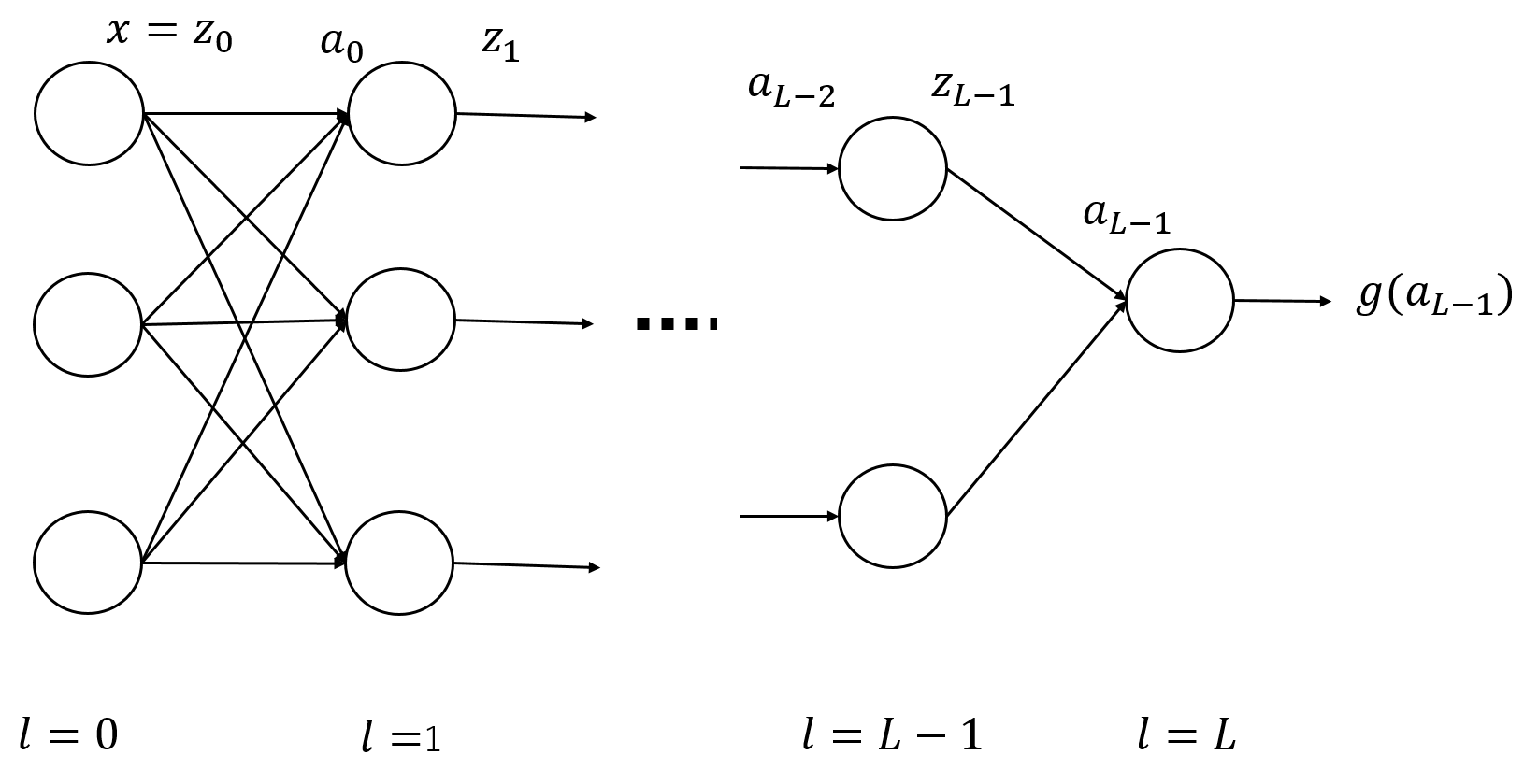
話を簡単にするため、層をまたいだ結合(skip-layer connection)はない、つまり、各素子は隣り合う層の素子とのみ結合しているものとします。
この節では、上記のニューラルネットワークの入出力関係を表す函数を書き下します。具体的には、各層の入出力関係の合成で全体を表します。これにより各層の寄与を抽出することができ、後の節で勾配を計算するときに役立ちます。
1.2.1 素子の個数
$l \in \left\{ 0, 1, \dots, L \right\}$に対し、$n_l \in \mathbb{N}$を第$l$層の素子の個数とします。
特に、$n_0 = d$となります。
1.2.2 活性化函数
これまた話を簡単にするため、隠れ層($l=0, \dots, L-1$)の活性化函数は全て同一であり、
これを$h : \mathbb{R} \rightarrow \mathbb{R}$とします。
$h$はたとえばlogistic sigmoid函数や、tanh、ReLUなどが利用できます。
また、後の記法のために、$h^{(l)}$を次のように定義します:
$$
\begin{align}
h^{(l)} : \mathbb{R}^{n_l} \rightarrow \mathbb{R}^{n_l}, \ \
h^{(l)}(a) = (h(a_1), h(a_2), \dots, h(a_{n_l}))^T \ \in \mathbb{R}^{n_l}.
\end{align}
$$
出力層(第$L$層)の活性化函数を$g : \mathbb{R}^{n_L} \rightarrow \mathbb{R}^{n_L}$とします。
$g$の具体的な選択は問題によって様々ですが、たとえば、
- 2クラス分類に対しては$g$はロジスティックシグモイド函数、
- 多クラス分類に対しては、$g$はsoftmax函数、
- 回帰問題に対しては、$g$は恒等写像、にとられることが多いようです。
1.2.3 各層の入出力
$l = 0,1, \dots, L-1$に対して、第$l$層の入出力を次のように定義します。
- $z^{(l)} \in \mathbb{R}^{n_l}$ : 第$l$層の出力
- $a^{(l)} \in \mathbb{R}^{n_{l+1}}$ : 第$(l+1)$層への入力
また、最終層の出力を$y \in \mathbb{R}^{n_L}$と表します。
隠れ層の活性化函数は$h$、出力層の活性化函数は$g$であったので、
$$
\begin{align}
z^{(l)} &= h^{(l)}(a^{(l-1)}) \ \ (l = 0,1, \dots, L-1) \
y &= g(a^{(L-1)})
\end{align}
$$
となります3。
各素子に関するパラメーターを次のように定義します。
- $w^{(l)}_{i,j}$ : 第$l$層の$j$番目の要素からの出力が、第$(l+1)$層の$i$番目の要素に入力されるときの重み。($i = 0, 1, n_{l+1}-1$, $j=0,1, \dots, n_{l}-1$.
- $b^{(l)}_{i}$ : 第$l$層の$i$番目の要素への入力に足されるbias。
これらのパラメーターを、行列とベクトルでまとめて表すことにします:
- $w^{(l)} = (w^{(l)}_{i,j})_{i,j}$ ただし、$w^{(l)}$は$n_{l+1} \times n_{l}$行列
- $b^{(l)} = (b^{(l)}_{0}, b^{(l)}_{1}, \dots, b^{(l)}_{n_{l+1}-1})^T$,
すると、$a^{(l)}$を$z^{(l)}$を用いて次のように表すことができます4:
$$
\begin{align}
a^{(l)} = w^{(l)} z^{(l)} + b^{(l)}
\end{align}
$$
後で使うために、このアファイン変換を
$$
\begin{align}
A^{(l)}_{\theta^{(l)}} : \mathbb{R}^{n_{l}} \rightarrow \mathbb{R}^{n_{l+1}} , \ \ A^{(l)}_{\theta^{(l)} }(z) := w^{(l)}z + b^{(l)}
\end{align},
$$
と表し、$\theta^{(l)} := (w^{(l)}, b^{(l)})$としておきます。
1.2.4 ネットワーク全体の形
$f_{\theta} : \mathbb{R}^{n_0} \rightarrow \mathbb{R}^{n_L}$を、上記のニューラルネットワーク全体の入出力を表す函数とします。ただし、$\theta$はパラメーターを一括して表したものとします。
ここまでの定義より、$f_\theta$は次のように書くことができます:
$$
\begin{align}
f_{\theta} = g \circ A^{(L-1)}_{\theta^{(L-1)}} \circ h^{(L-1)} \circ A^{(L-2)}_{\theta^{(L-2)}} \circ \cdots
A^{(l+1)}_{\theta^{(l+1)}} \circ h^{(l+1)} \circ A^{(l)}_{\theta^{(l)}} \circ h^{(l)} \circ A^{(l-1)}_{\theta^{(l-1)}}
\circ \cdots \circ h^{(1)} \circ A^{(0)}_{\theta^{(0)}} .
\end{align}
$$
特に、$\theta^{(l)}$に着目して分解すると、
$$
\begin{align}
f_{\theta} = F^{(l)} \circ A^{(l)}_{\theta^{(l)}} \circ Z^{(l)}
\ \ (l = 0, \dots, L-1)
\end{align}
$$
$$
\begin{align}
F^{(l)} &:= g \circ A^{(L-1)}_{\theta^{(L-1)}} \circ h^{(L-1)} \circ A^{(L-2)}_{\theta^{(L-2)}} \circ \cdots
A^{(l+1)}_{\theta^{(l+1)}} \circ h^{(l+1)} \ \ (l = 0,1, \dots, L-2) \
F^{(L-1)} &:= g \
Z^{(l)} &:= h^{(l)} \circ A^{(l-1)}_{\theta^{(l-1)}} \circ \cdots \circ h^{(1)} \circ A^{(0)}_{\theta^{(0)}} \ \ (l = 1, \dots, L-1)\
Z^{(0)} &:= I
\end{align}
$$
ここで、$f_{\theta} = F^{(l)} \circ A^{(l)}_{\theta^{(l)}} \circ Z^{(l)}$において、$\theta^{(l)}$が現れるのは$A^{(l)}_{\theta^{(l)}}$に限られることに注意しましょう。これにより、次の節での勾配の計算をラクに行うことができます。
1.3 損失函数と勾配
1.3.1 損失函数
ニューラルネットワークの学習にあたっては、次の形の損失函数$E_{tot}$を最小化することにします。
$$
\begin{align}
E_{tot}(\theta) = \frac{1}{N} \sum_{n=1}^{N} E \left( f_{\theta}(x_n), t_n \right) + \frac{\lambda}{2N} \|\theta \|^2 ,
\end{align}
$$
- $\lambda$は正則化パラメーター、
- $E$は任意性がありますが、たとえば下記のように取ることが多いかと思います:
- 回帰問題に対しては、$E(y,t) = \frac{1}{2} \| y - t \|^2$など。
- 多クラス分類問題で出力層がsoftmaxを用いる場合は、$E(y,t) = -\sum_{k=0}^{C-1} t_k \log y_k$ (対数尤度の符号を反転させたもの)。
1.3.2 勾配
次に、損失函数の、$w$や$b$についての微分(勾配)を求めます。正則化項については明らかなので、ここでは損失函数の第1項のみを考えることにします。また、第1項はデータ点についての和の形になっているので、まずは1つのデータ点からの寄与$E(f_{\theta}(x), t)$の勾配を考えることにします。
損失函数と$f_{\theta}$の定義から、各$l = 0,1,\dots, L-1$, $i=0, 1, \dots, n_{l+1}-1$, $j=0, 1, \dots, n_{l}-1$に対して、次が成り立ちます5:
$$
\begin{align}
\frac{\partial}{\partial w^{(l)}_{i,j}} E \left( f_{\theta}(x), t \right) &= \delta^{(l)}_{i} Z^{(l)}_{j}(x) \
\frac{\partial}{\partial b^{(l)}_{i}} E \left( f_{\theta}(x), t \right) &= \delta^{(l)}_{i} \
\delta^{(l)}_{i} &:= \sum_{k=0}^{n_L-1} \left. \frac{\partial E}{\partial y_k} \right|_{y=f_{\theta}(x)} \cdot
\left. \frac{\partial F^{(l)}_{k}}{\partial a^{(l)}_{i}} \right|_{a^{(l)}= (A^{(l)} \circ Z^{(l)})(x) }
\end{align}
$$
従って、勾配を求めるためには、$\delta^{(l)}_{i}$を求めればOKということが分かります。
$\delta^{(l)}_{i}$は、第$(l+1)$層の$i$番目の要素への入力($a^{(l)}_{i}$)が変化したときに、損失函数がどの程度変化するかを表しています。
記法を簡単にするために、$\delta^{(l)}_{i}$ ($i=0,1, \dots, n_{l+1}-1$)をまとめて$\delta^{(l)}$と表すことにしましょう。
次の節では、この$\delta^{(l)}$を効率的に求める方法「誤差逆伝播法」について論じます。
1.3.3 誤差逆伝播法
誤差逆伝播法では、$\delta^{(l)}$を帰納的に計算していきます。$l=L-1$から初めて、「$\delta^{(l+1)}$の情報を用いて$\delta^{(l)}$を求める」という方式で、$l = L-2, \dots, 1, 0$と1つずつ計算を行います。
まず、$l=L-1$を考えましょう。$F^{(L-1)} = g$となるので、定義より
$$
\begin{align}
\delta^{(L-1)}_{i} = \sum_{k=0}^{n_L-1} \left. \frac{\partial E}{\partial y_k} \right|_{y=f_{\theta}(x)} \cdot
\left. \frac{\partial g_{k}}{\partial a^{(L-1)}_{i}} \right|_{a^{(L-1)}= (A^{(L-1)} \circ Z^{(L-1)})(x) }
\end{align}
$$
となります。この式は多くの場合、簡単に表すことが出来ます。
- 回帰問題などで$E(y,t) = \frac{1}{2} \| y - t \|^2$, $g(a) = a$としたときは、$\delta^{(L-1)}_{i} = (f_{\theta}(x) - t)_{i}$となります。
- 多クラス分類で$E(y,t) = -\sum_{k=0}^{d_{out}-1} t_k \log y_k$, $g_k(a) = \frac{e^{a_k}}{\sum_{m} e^{a_m}}$としたときは、$\delta^{(L-1)}_{i} = (f_{\theta}(x) - t)_{i}$となります。
次に、ある$l \leq L - 2$に対して$\delta^{(l+1)}$が得られたとしましょう。この情報を用いて、$\delta^{(l)}$を次のように求めることができます:
$$
\begin{align}
\delta^{(l)}_{i} = h'(a^{(l)}_{i}) \sum_{j=0}^{n_{l+2}-1} \delta^{(l+1)}_{j} w^{(l+1)}_{j,i}
\end{align}
$$
この式の詳しい導出はここでは省きますが、$F^{(l)} = F^{(l+1)} \circ A^{(l+1)}_{\theta^{(l+1)}} \circ h^{(l+1)}$という関係式を用いると容易に示すことが出来ます。
1.4 More on 誤差逆伝播法
ここまでで、コスト函数とその勾配を求めるための式を導出しました。ここではもう一歩進んで、数式から少し実装寄りの話をしたいと思います。
1.4.1 記法の変更
本題に入る前に、ここで記法の変更を行います。前の節では重み$w$とバイアス$b$を別々に扱っていましたが、これをそのまま実装するのはやや煩雑になりそうです。そこで、$w$と$b$をまとめて扱えるようにしたいと思います。具体的には、次の変数$W^{(l)}$を定義します:
$$
\begin{align}
W^{(l)}_{i,j} =
\begin{cases}
b^{(l)}_{i} & (j=0) \
w^{(l)}_{i,j-1} & (j = 1,2, \dots, n_{l})
\end{cases}
\ \ (i = 0,1, \dots,n_{l+1} -1 ) ,
\end{align}
$$
$W^{(l)}$は$n_{l+1} \times (n_{l}+1)$行列となります。
また、各層の出力の記法も変更しておきます。
$$
\begin{align}
\tilde{z}^{(l)}_{i} =
\begin{cases}
1 & (i=0) \
z^{(l)}_{i-1} & (i = 1, \dots, n_l)
\end{cases}
\end{align}
$$
これらの記法を用いると、
$$
\begin{align}
a^{(l)} &= W^{(l)} \tilde{z}^{(l)} \
\tilde{z}^{(l)} &=
\begin{pmatrix}
1 \
z^{(l)}
\end{pmatrix} \
\frac{\partial}{\partial W^{(l)}_{i,j}} E(f_{\theta}(x),t) &= \delta^{(l)}_{i} \tilde{z}^{(l)}_{j}
\end{align}
$$
と書けます。
これにより、$w$と$b$を別々に扱う必要がなくなりました。
1.4.2 勾配の具体的な計算方法(1つのデータ点について)
以上の準備の下で、1つのデータ点$(x, t)$に対して、$E(f_{\theta}(x),t)$とその勾配を求める方法を具体的に書き下しておきます。
- まず、各層に対する$a^{(l)}, z^{(l)}$と出力層の$y$を次のように計算します(forward propagation)
$$
\begin{align}
\tilde{z}^{(0)} &= (1,x^T)^T) \
a^{(l)} &= W^{(l)} \tilde{z}^{(l)} \ \ (l=0, 1, \dots, L-1) ,\
\tilde{z}^{(l)} &=
\begin{pmatrix}
1 \
h^{(l)}(a^{(l-1)})
\end{pmatrix}\ \ (l=1,\dots, L-1) \
y &= g(a^{(L-1)})
\end{align}
$$ - 次に、$\delta^{(L-1)}$を計算します。具体的な形は$E$や活性化函数の形に依存しますが、1.3.3節の例(多クラス分類+$g$がsoftmax+$E$がcross entropoy、または、回帰問題+$g$が恒等写像+$E$が二乗誤差函数)では、
$$
\begin{align}
\delta^{(L-1)}_i = (y - t)_i .
\end{align}
$$
となります(ここは後で実装するときは、userが函数を指定する形にしておきます。)。 - さて、ここから$\delta^{(l)}$ ($l= L-2, L-1, \dots, 1, 0$)を帰納的に計算していきます($i = 0,1, \dots, n_{l+1} - 1$):
$$
\begin{align}
\delta^{(l)}_{i} = h'(a^{(l)}_{i}) \sum_{j=0}^{n_{l+2}-1} \delta^{(l+1)}_{j} W^{(l+1)}_{j,i+1}
\end{align}
$$
ここで、変数を$w$から$W$に変更しているため、式が前の節と少し変わっていることに注意しましょう。 - 最後に、$\delta$を用いて勾配を計算します:
$$
\begin{align}
\frac{\partial}{\partial W^{(l)}_{i,j}} E(f_{\theta}(x),t) = \delta^{(l)}_{i} \tilde{z}^{(l)}_{j}
\end{align}
$$
1.5 勾配降下法による最適化
この記事では、損失函数の最小化に勾配降下法を用いることにします。
勾配降下法では、変数を目的函数の勾配の反対の方向に少しずつ更新していきます。具体的には、$f$を目的函数、$x$をその変数、更新の$n$ステップ目での変数を$x_n$とすると、
$$
\begin{align}
x_{n+1} = x_n - \alpha \nabla f(x_n)
\end{align}
$$
として$x_n$を更新していきます。ここで、$\alpha > 0$は学習率で、手で決めてやる必要があります6。
2 数式からコードへ
さて、理論パートはようやく終わったので、これから数式をコードに変換していきます。例によって、データ点についてのloopを直接書かなくて済むように、numpy arrayの演算を活用していきます。
2.1 概観
今回はコードが長くなるので、詳細に入る前に概要をざっくりと見ておきましょう。
- まず、2.2節で変数をリストアップし、理論パートの変数と対応づけておきます。加えて、変数の形を変換する函数を与えます。
- 次に、2.3節と2.4節でforward propagationを行う函数
fpropと誤差逆伝播法で$\delta$を求める関数bpropを定義します。2.5節では、fpropとbpropを利用して、コスト函数とその勾配を求める函数を書きます。 - 2.6節では、勾配降下法で函数の最小化を行う関数を定義します。
- 最後に、2.7節ではこれらの函数をまとめて(利用して)、ニューラルネットワークを表す
NeuralNetクラスを与えます。
2.2 変数とその変換
まず、ニューラルネットワークに属性として持たせる変数を定義し、理論パートの数式を対応づけておきます。
-
num_neurons: ($L+1$,) array,num_neurons[l]= $n_{l}$ with $n_{0} = d$. -
act_func: 隠れ層の活性化函数$h$ -
act_func_deriv: $h$の導函数 -
out_act_func: 出力層の活性化函数$g$ -
E: 損失函数の第1項を表す函数。具体的には、$\frac{1}{N} \sum_{n=0}^{N-1}E(y_n, t_n)$を計算する函数。 -
lam: 正則化パラメーター$\lambda$ -
W_matrices: ($L$,) array, withdtype='object',W_matrices[l][i, j]= $W^{(l)}_{i,j}$
次に、補助的な変数を定義しておきます7。
-
X: ($N, d_{in}$) array。入力データ。X[n, i]$= X_{n, i} :=(x_{n})_{i}$ -
C: int, クラスの種数。 -
y: ($N$,) array, ラベルのデータ。yの各要素は0,1, ... , C-1のいずれかとします。 -
T: ($N, d_{out}$) array. ラベルデータの1-of-C符号化。T[n, i]$= T_{n, i} := (t_{n})_{i}$ -
Y: ($N, d_{out}$) array.Y[n, i]= $Y_{n, i} := $ 入力$x_n$に対するニューラルネットワークの出力の第$i$成分。 -
A_matrices: ($L$,) array withdtype='object',A_matrices[l][n, i]= $A^{(l)}_{n, i}$ := (入力$x_n$に対する$a^{(l)}_{i}$)。$A^{(l)}$の形は$(N, n_{l+1})$となります。 -
Z_matrices: ($L$,) array, withdtype='object',z_matrices[l][n, i]= $Z^{(l)}_{n, i}$ := (入力$x_n$に対する$\tilde{z}^{(l)}_{i}$。$Z^{(l)}$の形は$(N, n_l+1)$となります。 -
D_matrices: ($L$,) array, withdtype='object',D_matrices[l][n, i]= $\Delta^{(l)}_{n,i} :=$ (データ点$(x_n, t_n)$に対する$\delta^{(l)}_{i}$)。$\Delta^{(l)}$ の形は$(N, n_{l+1})$となります。
以下に、これらの変数を扱うための変換を行う函数を書いておきます。
まずは、1-ofC符号化です。理論パートでははじめから1-of-C符号化されたラベルのデータ$t$を扱ってきましたが、実際の応用ではこの符号化を計算する必要があります。そこで、生のラベルのデータyから1-of-C符号化を計算する函数を与えておきます。
def calcTmat(y, C):
    '''
    This function generates the matrix T from the training label y and the number of classes C

    Parameters
    ----------
    y : 1-D numpy array
        The elements of y should be integers in [0, C-1]
    C : int
        The number of classes

    Returns
    ----------
    T : (len(y), C) numpy array
        T[n, c] = 1 if y[n] == c else 0
    '''
    N = len(y)
    T = np.zeros((N, C))
    for c in range(C):
        T[:, c] = (y == c)
    return T
次に、W_matricesの変換です。理論パートにあわせるために、W_matricesは「2-D arrayを並べた1-D arary」としてあります8。しかし、最適化を行う際には、パラメーターはベクトルとして実数値の1-D arrayとしたほうが扱いやすくなります。そこで、ここではW_matricesをベクトルに変換する函数reshape_mat2vecと、その逆の変換を行う函数reshape_vec2matを与えておきます。これらの函数は、後ほど、勾配ベクトルを変換するときにも用います。
def reshape_vec2mat(vec, num_neurons):
    '''
    vec : 1-D numpy array, dtype float
        Vector, which we will convert into an array of matrices
    num_neurons : 1-D array, dtype int
        An array representing the structure of a neural network
    '''
    L = len(num_neurons) - 1
    matrices = np.zeros(L, dtype='object')
    ind = 0
    for l in range(L):
        mat_size = num_neurons[l+1] * (num_neurons[l] + 1)
        matrices[l] = np.reshape(vec[ind: ind + mat_size], ( num_neurons[l+1], num_neurons[l] + 1) )
        ind += mat_size
    return matrices

def reshape_mat2vec(matrices, num_neurons):
    '''
    matrices : 1-D numpy array, dtype object
        An array of matrices (2-D numpy array), which we will convert into a flattened 1-D array of float.
    num_neurons : 1-D array, dtype int
        An array representing the structure of a neural network
    '''
    L = len(num_neurons) - 1
    vec = np.zeros( np.sum(num_neurons[1:]*(num_neurons[:L] + 1)) )
    ind = 0
    for l in range(L):
        mat_size = num_neurons[l+1]*(num_neurons[l] + 1)
        vec[ind:ind+mat_size] = np.reshape(matrices[l], mat_size)
        ind += mat_size
    return vec
2.3 forward propagation
この節では、forward propagationによってネットワークの出力を求める函数を書きます。後で用いるために、$a^{(l)}$や$z^{(l)}$も返す仕様にしておきます。
複数のデータ点を一括で扱うために上手く行列を用います。具体的には、隠れ層の入出力$A^{(l)}$、$Z^{(l)}$ ($l=0,1,\dots, L-1$)と、最終層の出力$Y$を次のように求めます。
$$
\begin{align}
Z^{(l)} &= \begin{cases}
\left(\boldsymbol{1}_{N}, X \right) & (l=0) \\
\left(\boldsymbol{1}_{N} , h\left(A^{(l-1)} \right)\right) & (l = 1, \dots, L-1) \end{cases} \
A^{(l)} &= Z^{(l)} {W^{(l)}}^{T} \
Y &= g(A^{(L-1)})
\end{align}
$$
ただし、$\boldsymbol{1}_N := (1, 1, \dots, 1)^T \in \mathbb{R}^{N}$です。
また、記法をやや乱用し、$h$と$g$は行列$A^{(l)}$の各要素に作用しているものとみなしています。
def fprop(W_matrices, act_func, out_act_func, X):
    '''
    This function performs forward propagation, and calculate input/output for each layer of a neural network.

    Parameters:
    ----------
    W_matrices : 1-D array, dtype='object'
        (L,) array, where W_matrices[l] corresponds to the parameters of l-th layer.
    act_func : callable
        activation function for hidden layers
    out_act_func : callable
        activation function for the final layer
    X : 2-D array
        (N,d) numpy array, with X[n, i] = i-th element of x_n

    Returns:
    ----------
    Z_matrices : 1-D array, dtype='object'
        Z_matrices[l] is 1-D array, which represents the output from the l-th layer.
    A_matrices : 1-D array, dtype='object'
        A_matrices[l] is 1-D array, which represents the input to the (l+1)-th layer.
    Y : 2-D array
        The final output of the neural network.
    '''
    L = len(W_matrices)
    N = len(X)
    Z_matrices = np.zeros(L, dtype='object')
    A_matrices = np.zeros(L, dtype='object')

    Z_matrices[0] = np.concatenate((np.ones((N, 1)), X), axis=1)
    A_matrices[0] = Z_matrices[0] @ (W_matrices[0].T)

    for l in range(1, L):
        Z_matrices[l] = np.concatenate((np.ones((N, 1)), act_func(A_matrices[l-1])), axis=1)
        A_matrices[l] = Z_matrices[l] @ (W_matrices[l].T)
    Y = out_act_func(A_matrices[L-1])

    return Z_matrices, A_matrices, Y
2.4 誤差逆伝播
ここでは、$\delta$を求める関数を与えます。具体的には、次のように計算を行います。
- まず、$\Delta^{(L-1)}$を求めます。1.3.3節で挙げた具体例では、$\Delta^{(L-1)} = Y - T$となります。しかし、一般には$\Delta^{(L-1)}$は$A^{(l)}$や$Z^{(l)}$にも依存する可能性があります。そこで、ここでの実装では、
d_final_layerを$\Delta^{(L-1)}$を求める函数として外から与えておきます。 - $\Delta^{(l)}$ ($l= L-2, L-1, \dots, 1, 0$)を以下のように帰納的に求めます:
$$
\begin{align}
\Delta^{(l)} = h'(A^{(l)}) \ast \left( \Delta^{(l+1)} (W^{(l+1)}\mathrm{[:, 1:]})\right),
\end{align}
$$
ここで、$(W^{(l+1)}\mathrm{[:, 1:]})$は$W^{(l)}$から最初の列を除いたものを表し、$\ast$は成分ごとの積を表します。
def bprop(W_matrices, act_func, act_func_deriv, out_act_func, Z_matrices, A_matrices, Y, T, d_final_layer):
    '''
    This function performs backward propagation and returns delta.

    Parameters
    ----------
    W_matrices : 1-D array, dtype='object'
        (L,) array, where W_matrices[l] corresponds to the parameters of l-th layer.
    act_func : callable
        activation function for hidden layers
    act_func_deriv : callable
        The derivative of act_func
    out_act_func : callable
        activation function for the final layer
    Z_matrices : 1-D array, dtype='object'
        Z_matrices[l] is 1-D array, which represents the output from the l-th layer.
    A_matrices : 1-D array, dtype='object'
        A_matrices[l] is 1-D array, which represents the input to the (l+1)-th layer.
    Y : 2-D array
        The final output of the neural network.
    T : 2-D array
        Array for the label data.
    d_final_layer : callable
        A function of Z_matrices, A_matrices, Y and T, which returns $delta^{(L-1)}$

    Returns
    ----------
    D_matrices : 1-D array
        D_matrices[l] is a 2-D array, where D_matrices[l][n, i] = $\Delta^{(l)}_{n, i}$

    '''
    L = len(W_matrices)
    D_matrices = np.zeros(L, dtype='object')

    D_matrices[L-1] = d_final_layer(Z_matrices, A_matrices, Y, T)
    for l in range(L-2, -1, -1):
        D_matrices[l] = act_func_deriv(A_matrices[l]) * ( D_matrices[l+1] @ W_matrices[l+1][:, 1:] )

    return D_matrices
2.5 損失函数と勾配
ここでは、損失函数と勾配を同時に与える函数を定義します9。
まず、損失函数の値は
$$
\begin{align}
E_{tot}(\theta) = \frac{1}{N} \sum_{n=1}^{N} E \left( f_{\theta}(x_n), t_n \right) + \frac{\lambda}{2N} \|\theta \|^2.
\end{align}
$$
で与えられます。
第1項の勾配は次のように求めることができます。
$$
\begin{align}
\frac{\partial}{\partial W^{(l)}_{i,j}} \frac{1}{N}\sum_{n=0}^{N-1} E(f_{\theta}(x_n),t_n)
&= \frac{1}{N}\sum_{n=0}^{N-1} \Delta^{(l)}_{n,i} Z^{(l)}_{n,j} \
&= \frac{1}{N} \left( \Delta^{(l)T} Z^{(l)} \right)_{i,j}
\end{align}
$$
def cost_and_grad(W_matrices, X, T, act_func, act_func_deriv, out_act_func, E, d_final_layer, lam):
    '''
    This function performs backward propagation and returns delta.

    Parameters
    ----------
    W_matrices : 1-D array, dtype='object'
        (L,) array, where W_matrices[l] corresponds to the parameters of l-th layer.
    X : 2-D array
        (N,d) numpy array, with X[n, i] = i-th element of x_n
    T : 2-D array
        Array for the label data.
    act_func : callable
        activation function for hidden layers
    act_func_deriv : callable
        The derivative of act_func
    out_act_func : callable
        activation function for the final layer
    E : callable
        A function representing the first term of the cost function
    d_final_layer : callable
        A function of Z_matrices, A_matrices, Y and T, which returns $delta^{(L-1)}$
    lam : float
        Regularization constant

    Returns
    ----------
    cost_val : float
        The value of the cost function
    grad_matrices : 1-D array, dtype object
        Array of 2-D matrices corresponding the gradient
    '''

    N = len(X)
    L = len(W_matrices)

    Z_matrices, A_matrices, Y = fprop(
        W_matrices=W_matrices,
        act_func=act_func,
        out_act_func=out_act_func,
        X=X)

    cost_val = E(Y, T) + lam/(2*N)*( np.sum( np.linalg.norm(W)**2 for W in W_matrices ) )

    D_matrices = bprop(
        W_matrices=W_matrices,
        act_func=act_func,
        act_func_deriv=act_func_deriv,
        out_act_func=out_act_func,
        Z_matrices=Z_matrices,
        A_matrices=A_matrices,
        Y=Y,
        T=T,
        d_final_layer=d_final_layer)

    grad_matrices = np.zeros(L, dtype='object')
    for l in range(L):
        grad_matrices[l] = D_matrices[l].T @ Z_matrices[l] / N + lam/N * W_matrices[l]

    return cost_val, grad_matrices
2.6 勾配降下法による最小化
既に述べたように、勾配降下法では、
$$
\begin{align}
x_{n+1} = x_n - \alpha \nabla f(x_n).
\end{align}
$$
のように変数$x$を更新していきます。
この実装では、次の停止基準を採用します:「前のステップと比べたときの函数値の減少がftol以下になったら停止する」10。
def minimize_GD(func_and_grad, x0, alpha=0.01, maxiter=1e4, ftol=1e-5):
    '''
    This function minimizes the given function using gradient descent method

    Parameters
    ----------
    func_and_grad : callable
        A function which returns the tuple (value of function to be minimized (real-valued), gradient of the function)
    x0 : 1-D array
        Initial value of the variable
    alpha : float
        Learning rate
    maxiter : int
        Maximum number of iteration
    ftol : float
        The threshold for stopping criterion. If the change of the value of function is smaller than this value, the iteration stops.

    Returns
    ----------
    result : dictionary
        result['x'] ... variable, result['nit'] ... the number of iteration, result['func']...the value of the function, result['success']... whether the minimization is successful or not
    '''
    nit = 0
    x = x0
    val, grad = func_and_grad(x)
    while nit < maxiter:
        xold = x
        valold = val
        x = x - alpha*grad
        val, grad = func_and_grad(x)
        nit += 1
        if abs(val - valold) < ftol:
            break
    success = (nit < maxiter)
    return {'x': x, 'nit':nit, 'func':val, 'success':success}
2.7 Neural Network
長い長い準備が終わって、ようやくニューラルネットワーク本体にたどりつきました。
まず、ニューラルネットに与える(defaultの)活性化函数などを定義しておきます。
ここでは多クラス分類問題を考えるので、隠れ層はlogistic sigmoid函数、最終層はsoftmaxを持たせ、損失函数の第1項としてはcross entropyを取ることにします。
def E(Y,T):
    N = len(Y)
    return -np.sum( T*np.log(Y) )/N

def softmax(x):
    x0 = np.max(x,axis=1)
    x0 = np.reshape(x0, (len(x0),1))
    tmp = np.sum(np.exp(x-x0),axis=1)
    return np.exp(x-x0)/np.reshape(tmp,(len(tmp),1))

def sigmoid(x):
    return 1.0/(1 + np.exp(-x))

def sigmoid_deriv(x):
    return np.exp(-x)/((1+np.exp(-x))**2)

def d_final_layer(Z, A, Y, T):
    return Y - T
では、これまでの準備を全て組合せて、NeuralNetクラスを定義しましょう。
class NeuralNet:
    def __init__(self, C, lam, num_neurons, act_func=sigmoid, act_func_deriv=sigmoid_deriv, out_act_func=softmax, E=E, d_final_layer=d_final_layer):
        self.C = C
        self.num_neurons = num_neurons
        self.L = len(num_neurons) - 1
        self.act_func = act_func
        self.act_func_deriv = act_func_deriv
        self.out_act_func = out_act_func
        self.E = E
        self.d_final_layer = d_final_layer
        self.lam = lam
        self.W_matrices = np.zeros(self.L,dtype='object')

    def fit(self, X, y, ep=0.01, alpha=0.01, maxiter=1e4, ftol=1e-5, show_message=False):
        '''
        Parameters
        ----------
        X : 2-D array
            (N,d) numpy array, with X[n, i] = i-th element of x_n
        y : 1-D numpy array
            The elements of y should be integers in [0, C-1]
        ep : float
            The maximum value of the initial weight parameter, which will be used for random initialization
        alpha : float
            Learning rate
        maxiter : int
            Maximum number of iteration
        ftol : float
            The threshold for stopping criterion. If the change of the value of function is smaller than this value, the iteration stops.
        show_message : bool
            If True, the result of the optimization is shown.
        '''
        T = calcTmat(y, self.C)
        def cost_and_grad_vec(x):
            val, grad_mat = cost_and_grad(
                W_matrices=reshape_vec2mat(x, num_neurons=self.num_neurons),
                X=X,
                T=T,
                act_func=self.act_func,
                act_func_deriv=self.act_func_deriv,
                out_act_func=self.out_act_func,
                E=self.E,
                d_final_layer=self.d_final_layer,
                lam=self.lam
            )
            grad_vec = reshape_mat2vec(matrices=grad_mat, num_neurons=self.num_neurons)
            return val, grad_vec
        tht0 = 2*ep*(np.random.random(np.sum(self.num_neurons[1:]*(self.num_neurons[:self.L]+1))) - 0.5)
        time_start = time.time()
        result = minimize_GD(
            func_and_grad=cost_and_grad_vec,
            x0=tht0,
            alpha=alpha,
            maxiter=maxiter,
            ftol=ftol
        )
        time_end = time.time()
        if show_message:
            print(f"success : {result['success']}")
            print(f"nit : {result['nit']}")
            print(f"func value : {result['func']}")
            print(f"calcualtion time : {time_end - time_start}seconds")
        self.W_matrices=reshape_vec2mat(vec=result['x'], num_neurons=self.num_neurons)

    def predict_proba(self, X):
        '''
        Parameters
        ----------
        X : 2-D array
            (N,d) numpy array, with X[n, i] = i-th element of x_n

        Returns
        ----------
        Y : 2-D array
            (len(X), self.C) array, where Y[n, c] represents the probability that the n-th instance belongs to c-th class
        '''
        Z_matrices, A_matrices, Y = fprop(
            W_matrices=self.W_matrices,
            act_func=self.act_func,
            out_act_func=self.out_act_func,
            X=X)
        return Y

    def predict(self, X):
        '''
        Parameters
        ----------
        X : 2-D array
            (N,d) numpy array, with X[n, i] = i-th element of x_n

        Returns
        ----------
        classes : 1-D numpy array
            (len(X), ) array, where classes[n] represents the predicted class to which the n-th instance belongs
        '''
        Y = self.predict_proba(X)
        return np.argmax(Y, axis=1)
3 実験
それでは、ここまでのコードを実行してみましょう。
3.1 Gradient check
まず、実際にデータを用いて学習する前に、誤差逆伝播法の実装にバグがないかを確かめてみることにしましょう11。
この節では、誤差逆伝播法で求めた勾配と、数値微分で求めた勾配を比較し、それらが整合することを確かめます。
数値微分では、微分を次のように数値的に近似することにします。
$$
\begin{align}
\frac{\partial E_{tot} }{\partial W^{(l)}_{i,j}} \simeq
\frac{ E_{tot}(W^{(l)}_{i,j}+\varepsilon) - E_{tot}(W^{(l)}_{i,j}-\varepsilon) }{2\varepsilon},
\end{align}
$$
ただし、$E_{tot}(W^{(l)}_{i,j}\pm\varepsilon)$は、$W$の$(l,i,j)$成分のみを$\varepsilon$だけ変化させ、他の成分は固定したときの値を表します。
また、$\varepsilon$は十分小さいとします。
下記の函数では、NeuralNetオブジェクトnnを受け取り、W_vecでの勾配を数値微分と誤差逆伝播で計算してその結果を比較します。
def grad_check(nn, W_vec, X, T, ep):
    num_params = len(W_vec)
    W_matrices = reshape_vec2mat(W_vec, nn.num_neurons)
    cost, grad_mat_bp = cost_and_grad(W_matrices, X, T, act_func=nn.act_func, act_func_deriv=nn.act_func_deriv, out_act_func=nn.out_act_func, E=nn.E, d_final_layer=nn.d_final_layer, lam=nn.lam)
    grad_vec_bp = reshape_mat2vec(grad_mat_bp, nn.num_neurons)

    grad_vec_num = np.zeros(num_params)
    for cnt in range(num_params):
        W_p = np.copy(W_vec)
        W_m = np.copy(W_vec)
        W_p[cnt] += ep
        W_m[cnt] -= ep
        cost_p, grad_p = cost_and_grad(reshape_vec2mat(W_p, nn.num_neurons), X, T, act_func=nn.act_func, act_func_deriv=nn.act_func_deriv, out_act_func=nn.out_act_func, E=nn.E, d_final_layer=nn.d_final_layer, lam=nn.lam)
        cost_m, grad_m = cost_and_grad(reshape_vec2mat(W_m, nn.num_neurons), X, T, act_func=nn.act_func, act_func_deriv=nn.act_func_deriv, out_act_func=nn.out_act_func, E=nn.E, d_final_layer=nn.d_final_layer, lam=nn.lam)
        grad_vec_num[cnt] = (cost_p - cost_m )/(2*ep)
    return np.linalg.norm(grad_vec_bp - grad_vec_num), grad_vec_bp, grad_vec_num
小さなニューラルネットワークと適当なW_vec, X, Tを用いて試してみました:
num_neurons = np.array([4, 3, 2])

L = len(num_neurons) - 1
dim_W = np.sum(num_neurons[1:] * (num_neurons[:L]+1))
nn = NeuralNet(C=3, lam=1.0, num_neurons=num_neurons)
W_vec = np.arange(0.0, dim_W, 1)
X = np.reshape(np.arange(0.0, 2*num_neurons[0], 1.0), (2, num_neurons[0]))
T = np.array([[1.0,0],[0,1]])
error, grad_vec_bp, grad_vec_num = grad_check(nn, W_vec, X, T, ep=0.0001)

print(np.linalg.norm(grad_vec_bp)**2)
print(np.linalg.norm(grad_vec_num)**2)
print(error)
結果は
958.749997375419
958.7499973563445
1.641231604721956e-09
とのことで、ほぼ一致していると考えられます。
3.2 Toy data
誤差逆伝播法のチェックも終わったことですし、いよいよデータを与えて学習・予測してみましょう。
まずは単純な2次元のtoy dataを用いてみます。
X, y = datasets.make_blobs(n_samples=200, n_features=2, centers=3)
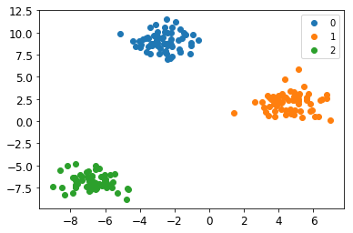
このデータを用いて、先ほどのNeuralNetを学習させます。ニューラルネットの形には(入力層と出力層の次元以外は)任意性がありますが、ここでは$L=2$, $n_0 = 2, n_1=3, n_2 = 3$と取ってみましょう。
clf = NeuralNet(C=3, lam=0.5, num_neurons=np.array([2, 2, 3]))
clf.fit(X, y, show_message=True, ep=0.1, alpha=0.1, ftol=1e-5)
結果はこちら
success : True
nit : 1295
func value : 0.130879514461342
calcualtion time : 0.40400195121765137seconds
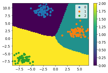
綺麗に分類できていることが見て取れるかと思います12。
3.3 手書き文字
学習と予測も問題なく動いていそうなことが分かりましたので、もう少し複雑なデータでも試してみましょう。
digits = datasets.load_digits()
dat_train, dat_test, label_train, label_test = train_test_split(digits.data, digits.target, test_size=0.25)
ここでも、ネットワークの構造にはだいぶ任意性がありますが、$L=2$、$n_0=64, n_1 = 35, n_2 = 10$と適当に取ってみたいと思います。
num_neurons = np.array([64,35,10])
nn_mnist = NeuralNet(C=10, lam=0.5, num_neurons=num_neurons)
nn_mnist.fit(dat_train, label_train, show_message=True, ep=0.01, alpha=0.1, ftol=1e-5)
結果は
success : True
nit : 2069
func value : 0.052294813440078226
calcualtion time : 6.497097730636597seconds
train accuracy score: 0.9985152190051967
test accuracy score: 0.9777777777777777
となりました。
こちらも適切に分類できているようです。
4 まとめ
今回は、全結合ニューラルネットワークによる多クラス分類を実装しました。定式化を整理しておさらいし、誤差逆伝播法などを行う函数を1つ1つ実装しました。最後にこれらを組合せてNeuralNetクラスを作成し、toy dataやMNIST手書き文字などを用いて、無事に動いていることを観察しました。
ただし、以下の課題が残りました:
- 重みの初期値や学習率、最適化の停止基準を変えると学習/予測の結果が大きく変わるケースが見られた。そのため、実際のデータに用いるには、複数の初期条件/設定での結果を簡単に比較/選択できるような機能があることが望ましい。
- ネットワーク構造を変えたときにどのような変化が起きるが、十分に観察できていない。
これらの課題については、また追々考えてみたいと思います。
-
たとえば、異なる層の$a_i$を区別していない点や、和において添え字が走る範囲が明確に書かれておらず誤解を招きやすい、など。 ↩
-
回帰や2クラス分類を含む定式化、という意味です。 ↩
-
ここで各素子の役割を定義している、というほうが正確ですが。 ↩
-
もしくは、これも「neural networkの重みとバイアスの定義」と言ったほうが正確かもしれません。 ↩
-
計算は省略してしまいますが、straightforwardな計算で示せます。 ↩
-
自動で決める方法もありますが、ここでは扱いません。気になる方は https://www.slideshare.net/pecorarista/steepest-descent などをご覧ください。 ↩
-
これはglobal変数として用いるという意味ではなく、原則として各函数の中のlocal変数でこういう名前の変数が出てきたときはこういう意味ですよ、という趣旨です。 ↩
-
それぞれの2-D arrayの形が異なるので、3-D arrayではかけません。 ↩
-
back propagationを行うにはforward propagationを行う必要があるので、函数の値を勾配を別々に計算するのは非効率化かと。 ↩
-
これだと学習率が小さすぎるとすぐに停止してしまうという問題があります。「勾配の値が0に十分近づいたら停止する」のほうが望ましいかもしれません。 ↩
-
Andrew Ng先生のCourseraの機械学習の講義でも推奨されていました。 ↩
-
なお、この例の場合、異なるクラスのデータ点どうしがかなり離れているせいか、学習率
alphaやftolを変えると決定境界が大きく変わるというふるまいが見られました。)。 ↩