Index
-----------------------Part-1-----------------------
- Introduction to Python Pandas
- Best Suitable for?
- Installing and Importing Pandas
- Creating a DataFrame in Pandas
- Reading and Writing Data with Pandas
- Data Selection and Indexing in Pandas
-----------------------Part-2-----------------------
7. Data Cleaning and Preprocessing with Pandas
8. Aggregation and Grouping with Pandas
9. Merging, Joining, and Concatenating DataFrames in Pandas
10. Time Series Analysis with Pandas
11. Visualization with Pandas
12. Conclusion and Next Steps
In this article, we will cover up to Index 6.
1. Introduction to Python Pandas
Pandas is a Python package providing fast, flexible, and expressive data structures designed to make working with “relational” or “labeled” data both easy and intuitive. It aims to be the fundamental high-level building block for doing practical, real world data analysis in Python. Additionally, it has the broader goal of becoming the most powerful and flexible open source data analysis / manipulation tool available in any language. It is already well on its way toward this goal.
Pandas is a high-level data manipulation tool developed by Wes McKinney. It is built on the Numpy package and its key data structure is called the DataFrame. DataFrames allow you to store and manipulate tabular data in rows of observations and columns of variables.
2. Best Suitable for?
Python Pandas is a versatile and powerful tool for data manipulation and analysis, and it can be suitable for a wide range of individuals and professions. Some of the groups who may find Pandas particularly useful include:
■Data Scientists and Analysts: Pandas provides a high-level, intuitive interface for working with data, making it a popular tool for data scientists and analysts who need to clean, transform, and analyze large datasets.
■Researchers: Researchers from various fields, such as economics, social sciences, and life sciences, often need to work with data. Pandas provides a convenient way to manage, manipulate, and analyze data, allowing researchers to focus on their research questions.
■Business Professionals: Business professionals, such as analysts, marketers, and product managers, can use Pandas to extract insights from data and make data-driven decisions.
■Programmers and Developers: Pandas is built on top of the Python programming language and can be easily integrated into Python code. Programmers and developers who work with data can use Pandas to create data-driven applications.
■Students: Students who are learning data science or programming can use Pandas to gain hands-on experience with real-world datasets.
In short, anyone who works with data or wants to learn more about data manipulation and analysis can benefit from using Python Pandas.
■Pandas is well suited for many different kinds of data:
・Tabular data with heterogeneously-typed columns, as in an SQL table or Excel spreadsheet
・Ordered and unordered (not necessarily fixed-frequency) time series data.
・Arbitrary matrix data (homogeneously typed or heterogeneous) with row and column labels
・Any other form of observational / statistical data sets. The data actually need not be labeled at all to be placed into a pandas data structure
■Here are just a few of the things that pandas does well:
・Easy handling of missing data (represented as NaN) in floating point as well as non-floating point data
・Size mutability: columns can be inserted and deleted from DataFrame and higher dimensional objects
・Automatic and explicit data alignment: objects can be explicitly aligned to a set of labels, or the user can simply ignore the labels and let Series, DataFrame, etc. automatically align the data for you in computations
・Powerful, flexible group by functionality to perform split-apply-combine operations on data sets, for both aggregating and transforming data
・Make it easy to convert ragged, differently-indexed data in other Python and NumPy data structures into DataFrame objects
・Intelligent label-based slicing, fancy indexing, and subsetting of large data sets
・Intuitive merging and joining data sets
・Flexible reshaping and pivoting of data sets
・Hierarchical labeling of axes (possible to have multiple labels per tick)
・Robust IO tools for loading data from flat files (CSV and delimited), Excel files, databases, and saving / loading data from the ultrafast HDF5 format
・Time series-specific functionality: date range generation and frequency conversion, moving window statistics, date shifting and lagging.
3. Installing and Importing Pandas
Installing Pandas
Pandas can be installed using pip, which is a package manager for Python.
pip install pandas
Importing Pandas
To load the pandas package and start working with it, import the package.
import pandas as pd
4. Creating a DataFrame in Pandas
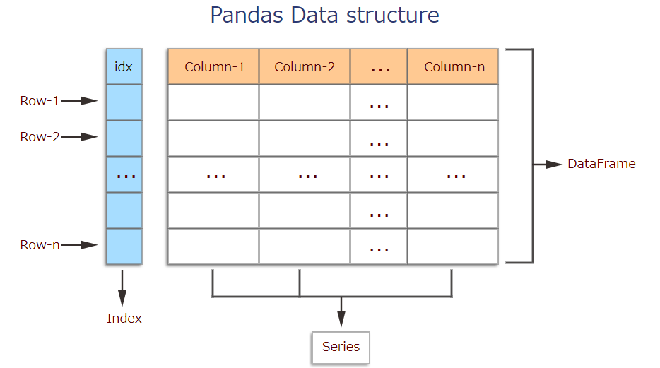
A DataFrame is a two-dimensional table-like data structure in Pandas. It contains an array of individual entries, each of which has a certain value. It can be created from various data sources, such as lists, dictionaries, CSV files, Excel files, and more
For example, consider the following simple DataFrame:
pd.DataFrame({'Yes': [50, 21], 'No': [131, 2]})
Output:
| Yes | No | |
|---|---|---|
| 0 | 50 | 131 |
| 1 | 21 | 2 |
DataFrame entries are not limited to integers. For instance, here's a DataFrame whose values are strings:
pd.DataFrame({'Bob': ['I liked it.', 'It was awful.'], 'Sue': ['Pretty good.', 'Bland.']})
Output:
| Bob | Sue | |
|---|---|---|
| 0 | I liked it. | Pretty good. |
| 1 | It was awful. | Bland. |
There are several ways to create a DataFrame. One way is to use a dictionary. For example:

・Series
A Series, by contrast, is a sequence of data values. If a DataFrame is a table, a Series is a list. And in fact you can create one with nothing more than a list:
pd.Series([1, 2, 3, 4, 5])
**Output:**
0    1
1    2
2    3
3    4
4    5
dtype: int64
5. Reading and Writing Data with Pandas
■Reading Data
Pandas can read data from various file formats, such as CSV, Excel, SQL, JSON, and more.
It's another way to create a DataFrame is by importing a csv file using Pandas.
Data can be stored in any of a number of different forms and formats. By far the most basic of these is the humble CSV file. Now, the csv cars.csv is stored and can be imported using pd.read_csv:

or we can examine the contents of the resultant DataFrame using the head() command, which grabs the first five rows:
pd.head()
■Writing Data
Pandas can write data to various file formats as well, such as CSV, Excel, SQL, JSON, and more. Here's an example of writing data to a CSV file:
import pandas as pd

# create a DataFrame
df = pd.DataFrame({'Name': ['Alice', 'Bob', 'Charlie'],
                   'Age': [25, 30, 35],
                   'City': ['New York', 'Paris', 'London']})

# write data to a CSV file
df.to_csv('data.csv', sep=';', header=True,  index=False)
That's it for reading and writing data with Pandas! Once you can read and write data, you can start using Pandas to manipulate and analyze data.
6. Data Selection and Indexing in Pandas
6.1 Selecting Data by Column
import pandas as pd

# create a DataFrame
df = pd.DataFrame({'Name': ['Alice', 'Bob', 'Charlie'],
                   'Age': [25, 30, 35],
                   'City': ['New York', 'Paris', 'London']})

# select a column by name
name_col = df['Name']
In this example, we use the [] operator to select the "Name" column in the DataFrame df. The resulting data is stored in a Series name_col.
6.2 Selecting Data by Row
import pandas as pd

# create a DataFrame
df = pd.DataFrame({'Name': ['Alice', 'Bob', 'Charlie'],
                   'Age': [25, 30, 35],
                   'City': ['New York', 'Paris', 'London']})

# select a row by index using .loc[]
alice_row = df.loc[0]

# select a row by integer index .iloc[]
bob_row = df.iloc[1]
In this example, we use the .loc[] operator to select the first row in the DataFrame df and store the resulting data in a Series alice_row. We also use the .iloc[] operator to select the second row in the DataFrame df and store the resulting data in a Series bob_row.
6.3 Selecting Data by Condition
import pandas as pd

# create a DataFrame
df = pd.DataFrame({'Name': ['Alice', 'Bob', 'Charlie'],
                   'Age': [25, 30, 35],
                   'City': ['New York', 'Paris', 'London']})

# select rows where Age is greater than 30
age_gt_30 = df[df['Age'] > 30]
In this example, we use boolean indexing to select the rows in the DataFrame df where the "Age" column is greater than 30. The resulting data is stored in a new DataFrame age_gt_30.
6.4 Indexing Data
import pandas as pd

# create a DataFrame
df = pd.DataFrame({'Name': ['Alice', 'Bob', 'Charlie'],
                   'Age': [25, 30, 35],
                   'City': ['New York', 'Paris', 'London']})

# set "Name" column as index
df.set_index('Name', inplace=True)

# index data using .loc[]
alice_age = df.loc['Alice', 'Age']

# index data using .iloc[]
bob_age = df.iloc[1, 1]
In this example, we use the .set_index() method to set the "Name" column as the index of the DataFrame df. We then use the .loc[] operator to index the "Age" value of the row with index "Alice" and store it in a variable alice_age. We also use the .iloc[] operator to index the "Age" value of the row with index 1 (i.e., "Bob") and column index 1 (i.e., "Age") and store it in a variable bob_age.
Other Useful Tricks
・Get the current working directory
import os
os.getcwd()
・Check how many rows and columns present in the data
pd.shape
Output:
(no. of rows, no. of columns)
(2200, 15)
・Rename the columns
pd_new = pd.rename(colums = {'Amount.Requested': 'Amount.Requested_NEW'})
pd_new.head()
here is the cheat-sheet for pandas.
https://pandas.pydata.org/Pandas_Cheat_Sheet.pdf
Enjoy the Power of Pandas and I hope you found it helpful.
Thank you for spending the time to read this article.
See you in Part-2 topics. ![]()
![]()
Thank you.


