Automated Machine Learning(@Azure ML)を試す

Auto ML（Automated Machine Learning）とは

以下、Automate Machine Learningに関する日本語資料が乏しいため色んなサイトを
漁って意訳して回りました。

Automate Machine Learning（以下AML）とは現実世界の課題を機械学習に適応させる二者間の自動化プロセスである。
AMLはこれまで予測パフォーマンスの最大化を目的として専門家、熟練者が行ってきた前処理、特徴量抽出、特徴量選択、モデル選択を自動化する。
これらは熟練者でないスタッフには不可能でAMLはますます増加する課題解決に対する機械学習の適用に対するAIベースのソリューションとして提案された。
AMLはよりシンプルで迅速、また手作業よりもよりすぐれた性能を発揮するプロダクトの生産を提供する。

機械学習の民主化

真っ先に「技術はまず最初にデータサイエンティストの仕事を奪うのか？」という考えが過った。
高い精度の追及は進捗を遅延させ、または他のプロジェクトへの参画を不可能にする。もしくは別の選択肢として精度を低くすると他のことに使う時間を作ることができる。
そして機械学習は作ったら終わりではなくデータが発展するに連れ、スパムや詐称の検知、天気に依存するモデル等、メンテナンスも必要になる。現在抱えているソリューションの維持と新たな問題へのデータサイエンティストとしての対応で時間が全くない。
AMLは生産性のあるツールとしてデータサイエンティストに力を与える。もしくは専門家がいようといまいと、モデルに高い精度を与え、専門家が行うよりも少ない時間で前処理からチューニングに至るまでの機械学習による一連の解決方法を顧客に識別させる。機械学習の民主化である。

データに触れない？

データサイエンティストがデータを除いて解析する機会も少なくなる。データサイエンティストや開発者は顧客の持つデータのプライバシーを保護しデータに触れることなくデータをAMLに投入、前処理から検証に至るまでを自動化できる。

何をautomateするのか

もちろん、製品により異なるが自動化の対象は前処理だけでなく多岐に渡り概ね以下のようなものがある。

• 生データからの学習対象データの取得、データのタイプ、意図、タスクの発見の自動化
• 特徴量抽出、選択、メタ学習、転移学習
• 異常値の発見、欠損値への対応
• モデルの選択
• ハイパーパラメータの最適化
• 結果の分析と問題の発見
• AMLの可視化

⇒つまり作業の全部。もしくはこれからすべてが対象になる可能性がある。

プロダクト・ライブラリ

Auto-WEKA
Java製の統計解析ツール。「集合知 in Action」で知った方も多いのでは。

auto-Sklearn
scikit-learnの自動化ライブラリ。下記Azure MLの多くがscikit-learnのライブラリを使用しています。

Automated Machine Learning(Microsoft )
Microsoft Ignite 2018にてAzure MLとの統合が発表された。現在preview版で利用可能。

Google Cloud AutoML
GCPのサービス。AutoML Translation、Natural Language、Vision がベータ版で利用可能。

karura
個人開発のようで早い段階で取り組まれているようです。モデルの選択はskLearnのチャートを利用されています

Azure Automated Machine Learningによる機械学習の自動化

ここからは先はMicrosoft Azure MLのAutomated Machine Learningのお話になります。
チュートリアルとサンプルをベースに自動化を実行してみました。
今回の記事執筆時まだAzureの公式サイトで和訳されたものがなかったのですが
2018/10/10に再度確認したところチュートリアルが和訳されていました。

チュートリアル: Azure Machine Learning の自動機械学習で分類モデルをトレーニングする

jupyter notetbook上で実行しますがAzure jupyter notebookを利用する方法と、ローカルのnotebookでの実行の２通りあります。
今回は後者で試してみたいと思います。
またソースはほぼほぼサンプルソースの実行となります。
サンプルではデータを事前に用意する必要もありません。
が、通常の作業時はautomateと言っても行うことが大きく以下２点あります。

• データの投入
• 設定値の準備

利用できるアルゴリズム

アルゴリズムのカテゴリ（分類or回帰）を選択する必要がありますが、
アルゴリズムの選択は自動化してくれます。
サポートされているアルゴリズムは以下となります。

分類

• ロジスティック回帰
• 確率的勾配降下法
• ナイーブベイズ（ベルヌーイモデル）
• ナイーブベイズ（多項式モデル）
• サポートベクターマシーン
• LinearSVC
• CalibratedClassifierCV
• 決定木
• K近傍法
• 確率的勾配降下法
• ランダムフォレスト
• Extra-Trees
• LGBM

回帰

• Elastic Net回帰
• 勾配ブースティング回帰
• 決定木
• K近傍法
• LARS-lasso
• 確率的勾配降下法
• ランダムフォレスト
• Extra-Trees
• LGBM

ローカルのnotebookでAutomated Machine Learningを実行

python3.6での実装です。

必要なモジュールのインストール + インポート

必要に応じてインストールします
jupyter notebook→ pip install azureml
azure jupyter notebook→ !pip install azureml

import logging
import os
import random

from matplotlib import pyplot as plt
from matplotlib.pyplot import imshow
import numpy as np
import pandas as pd
from sklearn import datasets

import azureml.core
from azureml.core.experiment import Experiment
from azureml.core.workspace import Workspace
from azureml.train.automl import AutoMLConfig
from azureml.train.automl.run import AutoMLRun

Azure MLのワークスペースを作成

createメソッドでワークスペースを作成します。

# ワークスペース作成
ws = Workspace.create(
    name='myworkspace',
    subscription_id='bxxxxxx27-2xx5-4xxx3-8dx4-f3xxxxxxx1',
    resource_group='VXXXXXXL',
    create_resource_group='false',
    location='xxxxxxxxxxxx'
)
# 作成内容の表示
ws.get_details()
experiment_name = 'automl-local-regression'
project_folder = './sample_projects/automl-local-regression'

experiment = Experiment(ws, experiment_name)

output = {}
output['SDK version'] = azureml.core.VERSION
output['Subscription ID'] = ws.subscription_id
output['Workspace Name'] = ws.name
output['Resource Group'] = ws.resource_group
output['Location'] = ws.location
output['Project Directory'] = project_folder
output['Experiment Name'] = experiment.name
pd.set_option('display.max_colwidth', -1)
pd.DataFrame(data = output, index = ['']).T

作成したワークスペースは以下のように読み込むことが出来ます。

Workspace.from_config()

Azure 診断拡張機能

from azureml.telemetry import set_diagnostics_collection
set_diagnostics_collection(send_diagnostics = True)

データの読み込み

sklearnからdatasetを拝借する
sklearn.datasets.load_diabetes

from sklearn.datasets import load_diabetes
from sklearn.linear_model import Ridge
from sklearn.metrics import mean_squared_error
from sklearn.model_selection import train_test_split

# 既存データの読み込み
X, y = load_diabetes(return_X_y = True)

columns = ['age', 'gender', 'bmi', 'bp', 's1', 's2', 's3', 's4', 's5', 's6']

# テストデータ分割
X_train, X_test, y_train, y_test = train_test_split(X, y, test_size = 0.2, random_state = 0)

AutoMLの設定

AutoMLで行う主たる作業はここになるかと思います。
自動化の設定内容です。
現在把握している設定値は以下のようなものです。

設定項目名	設定内容
task	回帰か分類かを指定
primary_metric	優先指標
max_time_sec	イテレーションの秒単位での上限値
iterations	イテレーション回数
n_cross_validations	交差検証時分割数
debug_log	ログのパス
verbosity	ログレベル
x	説明変数
y	目的変数
preprocess	前処理を行うか否か(true/false)
exit_score	終了する上限値（この値に到達すれば完了）
blacklist_algos	除外する手法をカンマ区切りで列挙

automl_config = AutoMLConfig(task = 'regression',
                             max_time_sec = 600,
                             iterations = 10,
                             primary_metric = 'spearman_correlation',
                             n_cross_validations = 5,
                             debug_log = 'automl.log',
                             verbosity = logging.INFO,
                             X = X_train, 
                             y = y_train,
                             path = project_folder)

train + verify を依頼

experimentオブジェクトのsubmitメソッドで上記設定内容を送信します。
その後最適なモデルの選択が検証されます。
このフェーズでおよそ5分程かかりました。

local_run = experiment.submit(automl_config, show_output = True)

結果表示

***********************************************************************************************
ITERATION: The iteration being evaluated.
PIPELINE: A summary description of the pipeline being evaluated.
DURATION: Time taken for the current iteration.
METRIC: The result of computing score on the fitted pipeline.
BEST: The best observed score thus far.
***********************************************************************************************

 ITERATION     PIPELINE                               DURATION                METRIC      BEST
         0      StandardScalerWrapper LightGBMRegresso0:00:28.641397           0.669     0.669
         1      MaxAbsScaler LightGBMRegressor        0:00:24.636259           0.682     0.682
         2      StandardScalerWrapper SGDRegressor    0:00:19.451089           0.639     0.682
         3      TruncatedSVDWrapper KNeighborsRegresso0:00:18.586640           0.566     0.682
         4      MaxAbsScaler ExtraTreesRegressor      0:00:18.044196           0.673     0.682
         5      SparseNormalizer RandomForestRegressor0:00:17.551055           0.697     0.697
         6      MaxAbsScaler DecisionTreeRegressor    0:00:19.553219           0.385     0.697
         7      MaxAbsScaler KNeighborsRegressor      0:00:17.916087           0.648     0.697
         8      StandardScalerWrapper ExtraTreesRegres0:00:20.786950           0.699     0.699
         9      MaxAbsScaler SGDRegressor             0:00:18.151557           0.002     0.699

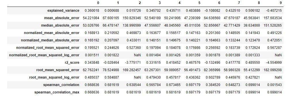
詳細結果表示

# 保持している詳細情報をget_children()でfetchして表示
from azureml.train.widgets import RunDetails
RunDetails(local_run).show() 
children = list(local_run.get_children())
metricslist = {}

for run in children:
    properties = run.get_properties()
    metrics = {k: v for k, v in run.get_metrics().items() if isinstance(v, float)}
    metricslist[int(properties['iteration'])] = metrics

rundata = pd.DataFrame(metricslist).sort_index(1)
rundata

結果表示

最適モデルの検索

ExtraTreesRegressor

best_run, fitted_model = local_run.get_output()
print(best_run)
print(fitted_model)

結果表示

Run(Experiment: automl-local-regression,
Id: AutoML_817085d1-e775-4726-a039-43931b89fdef_8,
Type: None,
Status: Completed)
Pipeline(memory=None,
     steps=[('StandardScalerWrapper', <azureml.train.automl.model_wrappers.StandardScalerWrapper object at 0x0000029A545E8F98>), ('ExtraTreesRegressor', ExtraTreesRegressor(bootstrap=True, criterion='mse', max_depth=None,
          max_features=None, max_leaf_nodes=None,
          min_impurity_decrease=0...timators=100, n_jobs=1,
          oob_score=False, random_state=None, verbose=0, warm_start=False))])

最適なモデルをテスト

y_pred_train = fitted_model.predict(X_train)
y_residual_train = y_train - y_pred_train

y_pred_test = fitted_model.predict(X_test)
y_residual_test = y_test - y_pred_test

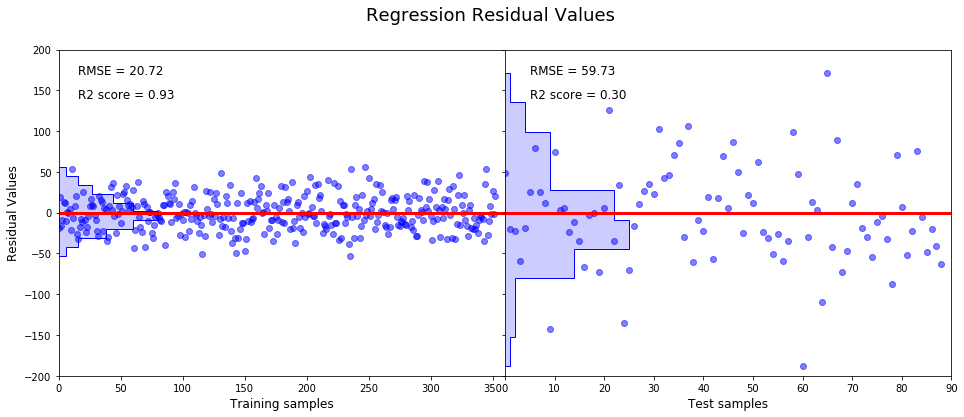
プロット

頂き物のサンプルソースで描画

%matplotlib inline
import matplotlib.pyplot as plt
import numpy as np
from sklearn import datasets
from sklearn.metrics import mean_squared_error, r2_score

# Set up a multi-plot chart.
f, (a0, a1) = plt.subplots(1, 2, gridspec_kw = {'width_ratios':[1, 1], 'wspace':0, 'hspace': 0})
f.suptitle('Regression Residual Values', fontsize = 18)
f.set_figheight(6)
f.set_figwidth(16)

# Plot residual values of training set.
a0.axis([0, 360, -200, 200])
a0.plot(y_residual_train, 'bo', alpha = 0.5)
a0.plot([-10,360],[0,0], 'r-', lw = 3)
a0.text(16,170,'RMSE = {0:.2f}'.format(np.sqrt(mean_squared_error(y_train, y_pred_train))), fontsize = 12)
a0.text(16,140,'R2 score = {0:.2f}'.format(r2_score(y_train, y_pred_train)), fontsize = 12)
a0.set_xlabel('Training samples', fontsize = 12)
a0.set_ylabel('Residual Values', fontsize = 12)

# Plot a histogram.
a0.hist(y_residual_train, orientation = 'horizontal', color = 'b', bins = 10, histtype = 'step');
a0.hist(y_residual_train, orientation = 'horizontal', color = 'b', alpha = 0.2, bins = 10);

# Plot residual values of test set.
a1.axis([0, 90, -200, 200])
a1.plot(y_residual_test, 'bo', alpha = 0.5)
a1.plot([-10,360],[0,0], 'r-', lw = 3)
a1.text(5,170,'RMSE = {0:.2f}'.format(np.sqrt(mean_squared_error(y_test, y_pred_test))), fontsize = 12)
a1.text(5,140,'R2 score = {0:.2f}'.format(r2_score(y_test, y_pred_test)), fontsize = 12)
a1.set_xlabel('Test samples', fontsize = 12)
a1.set_yticklabels([])

# Plot a histogram.
a1.hist(y_residual_test, orientation = 'horizontal', color = 'b', bins = 10, histtype = 'step')
a1.hist(y_residual_test, orientation = 'horizontal', color = 'b', alpha = 0.2, bins = 10)

plt.show()