
こちらの記事は,ロボティクスの辞書的な記事(にしたい記事)のコンテンツです.
- 事前に必要な知識(見ておいた方が良い記事)
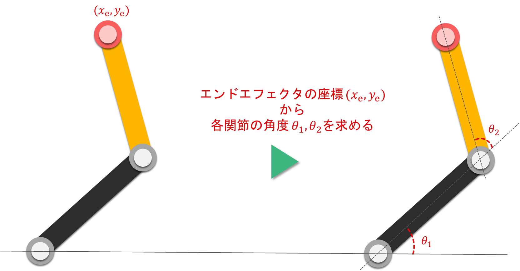
この記事では「解析的な逆運動学の解法」について解説していきたいと思います
逆運動学は、
「エンドエフェクタの位置、姿勢」から「各関節の角度」
を求めますが、その中でも解析的解法は
解析的な方法で「エンドエフェクタの位置,姿勢」から「各関節の角度」を求める
ことになります。
なお。本記事内のコードはすべてgoogle colaboratory上でも動作します(2023/10/26現在)。
💡 本記事に出てくるコードはnotebook上で動作させる(「ipynb」ファイル)ことを前提としているため「py」ファイルでは一部のコードは動作しないのでご注意ください(主に描画関連)
解析的解法のメリット·デメリット
解析的解法のメリットとしては
- 一度、数式を求めることができれば、一瞬で解が求まる
- 幾何的に求めるため、精度が高い
といった点があります
一方で、デメリットとしては
- ロボットアームの軸数が増加すると、 数式が複雑になる(ロボットの構成によっては、解析的解法では逆運動学が解けない場合もある)
といった点が挙げられます。
例:2軸の回転関節を持ったロボットアームの解析的解法による逆運動学
今回は、「三角関数による順運動学」の解説にも使用した
2軸の回転関節を持ったロボットアーム
を用いて解析的に逆運動学を解く手順を解説します。
解析的解法には、以下の二種類の解法が存在します。
- 代数的に求める方法
- 幾何学的に求める方法
ここからは、「三角関数による順運動学」が理解できている前提で話を進めていきます
方法1)代数的に求める
最初に、「三角関数による順運動学」の「各関節の角度 から エンドエフェクタの位置」を求める数式を再度確認してみましょう
\begin{align}
x_{\mathrm{e}}&=L_1\cos(\theta_1)+L_2\cos(\theta_1+\theta_2) \tag{1}\\
\end{align}
\begin{align}
y_{\mathrm{e}}&=L_1\sin(\theta_1)+L_2\sin(\theta_1+\theta_2)\tag{2}\\
\end{align}
式(1)(2)は
各関節の角度 から エンドエフェクタの位置 を求めていますが、
この式を変形すれば
エンドエフェクタの位置 から 各関節の角度
を求めることができます。
ここからは式(1)(2)を式変形していき、各課関節の角度を導出していきます。
\begin{align}
x_{\mathrm{e}}&=L_1\cos(\theta_1)+L_2\cos(\theta_1+\theta_2) \tag{1}\\
\end{align}
\begin{align}
y_{\mathrm{e}}&=L_1\sin(\theta_1)+L_2\sin(\theta_1+\theta_2) \tag{2}
\end{align}
式(1)(2) を 式(1’)(2’) に変換します。
\begin{align}
x_{\mathrm{e}} - L_1\cos(\theta_1) &= L_2\cos(\theta_1+\theta_2) \tag{1'}\\
\end{align}
\begin{align}
y_{\mathrm{e}}- L_1\sin(\theta_1)&=L_2\sin(\theta_1+\theta_2) \tag{2'}
\end{align}
式(1’)(2’) の両辺を2乗します。
\begin{align}
(x_{\mathrm{e}} - L_1\cos(\theta_1))^2 &= (L_2\cos(\theta_1+\theta_2))^2 \\
x_{\mathrm{e}}^2 - 2x_{\mathrm{e}}L_1\cos(\theta_1)+L_1^2 \cos^2(\theta_1) &= L_2^2\cos^2(\theta_1+\theta_2)
\tag{1''}
\end{align}
\begin{align}
(y_{\mathrm{e}} - L_1\sin(\theta_1))^2 &= (L_2\sin(\theta_1+\theta_2))^2\\
y_{\mathrm{e}}^2 - 2y_{\mathrm{e}}L_1\sin(\theta_1)+L_1^2 \sin^2(\theta_1) &= L_2^2\sin^2(\theta_1+\theta_2)
\tag{2''}\\
\end{align}
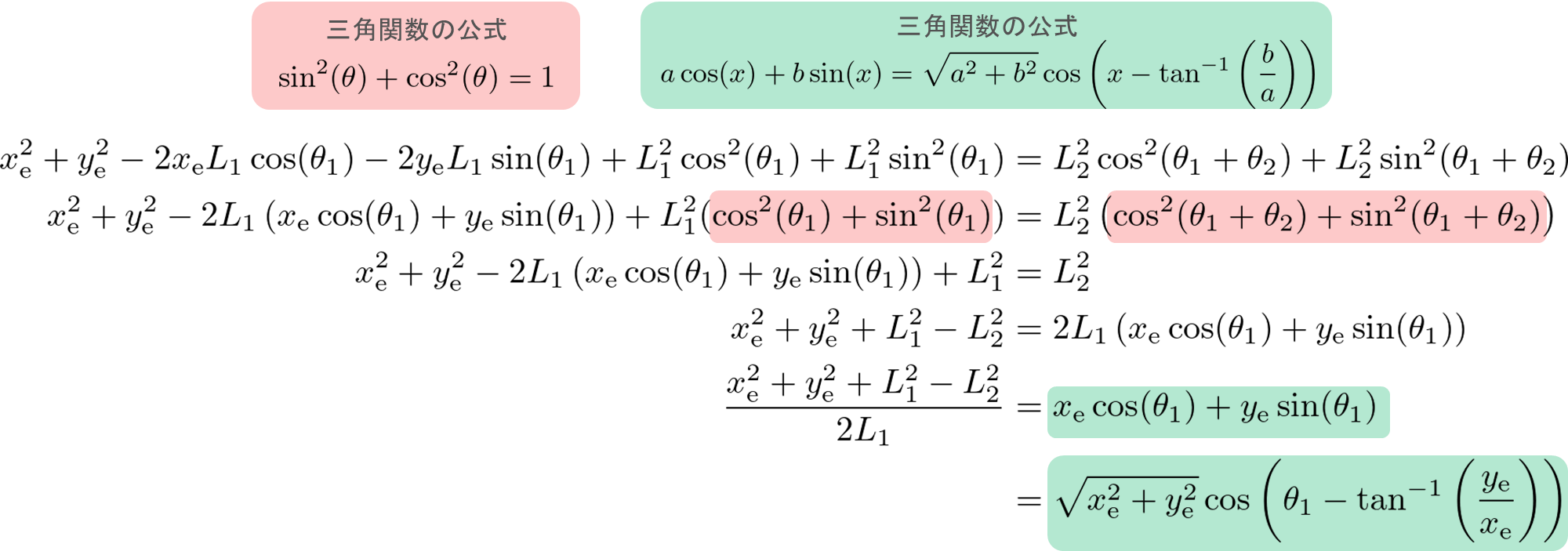
式(1’’)と式(2’’)を足します
\begin{align}
x_{\mathrm{e}}^2  + y_{\mathrm{e}}^2- 2x_{\mathrm{e}}L_1\cos(\theta_1) - 2y_{\mathrm{e}}L_1\sin(\theta_1) +L_1^2 \cos^2(\theta_1) +L_1^2 \sin^2(\theta_1)&= L_2^2\cos^2(\theta_1+\theta_2)+L_2^2\sin^2(\theta_1+\theta_2)\\

x_{\mathrm{e}}^2  + y_{\mathrm{e}}^2 - 2L_1\left(x_{\mathrm{e}}\cos(\theta_1\right) + y_{\mathrm{e}}\sin(\theta_1)) +L_1^2(\cos^2(\theta_1) +\sin^2(\theta_1))&= L_2^2\left(\cos^2(\theta_1+\theta_2)+\sin^2(\theta_1+\theta_2)\right)\\

x_{\mathrm{e}}^2  + y_{\mathrm{e}}^2 - 2L_1\left(x_{\mathrm{e}}\cos(\theta_1\right) + y_{\mathrm{e}}\sin(\theta_1)) +L_1^2&= L_2^2\\


x_{\mathrm{e}}^2  + y_{\mathrm{e}}^2 + L_1^2  -L_2^2   &= 2L_1\left(x_{\mathrm{e}}\cos(\theta_1\right) +y_{\mathrm{e}}\sin(\theta_1))\\

\frac{x_{\mathrm{e}}^2  + y_{\mathrm{e}}^2 + L_1^2  -L_2^2   }{2L_1}&= x_{\mathrm{e}}\cos(\theta_1) +y_{\mathrm{e}}\sin(\theta_1)\\

&= \sqrt{x_{\mathrm{e}}^2+y_{\mathrm{e}}^2}\cos \left(\theta_1 - \tan^{-1} \left(\frac{ y_{\mathrm{e}} }{ x_{\mathrm{e} }}\right)\right)

\tag{3}
\end{align}
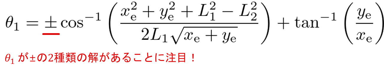
ここで、式(3)を $\theta_1$ について解くと
\begin{align}

\frac{x_{\mathrm{e}}^2  + y_{\mathrm{e}}^2 + L_1^2  -L_2^2   }{2L_1} &= \sqrt{x_{\mathrm{e}}^2+y_{\mathrm{e}}^2}\cos \left(\theta_1 - \tan^{-1} \left(\frac{ y_{\mathrm{e}} }{ x_{\mathrm{e} }}\right)\right) \tag{4}\\


\frac{x_{\mathrm{e}}^2  + y_{\mathrm{e}}^2 + L_1^2  -L_2^2   }{2L_1 \sqrt{x_{\mathrm{e}}^2+y_{\mathrm{e}}^2}}
&=
\cos \left(\theta_1 - \tan^{-1} \left(\frac{ y_{\mathrm{e}} }{ x_{\mathrm{e} }}\right)\right)\\

\pm\cos^{-1}\left(\frac{x_{\mathrm{e}}^2  + y_{\mathrm{e}}^2 + L_1^2  -L_2^2   }{2L_1 \sqrt{x_{\mathrm{e}}^2+y_{\mathrm{e}}^2}}\right)
&=
\theta_1 - \tan^{-1} \left(\frac{ y_{\mathrm{e}} }{ x_{\mathrm{e} }}\right)\\

\theta_1
&=
\pm\cos^{-1}\left(\frac{x_{\mathrm{e}}^2  + y_{\mathrm{e}}^2 + L_1^2  -L_2^2   }{2L_1 \sqrt{x_{\mathrm{e}}^2+y_{\mathrm{e}}^2}}\right) + \tan^{-1} \left(\frac{ y_{\mathrm{e}} }{ x_{\mathrm{e} }}\right)
\\

\tag{3}
\end{align}
となり、1つ目の角度を求めることができました。
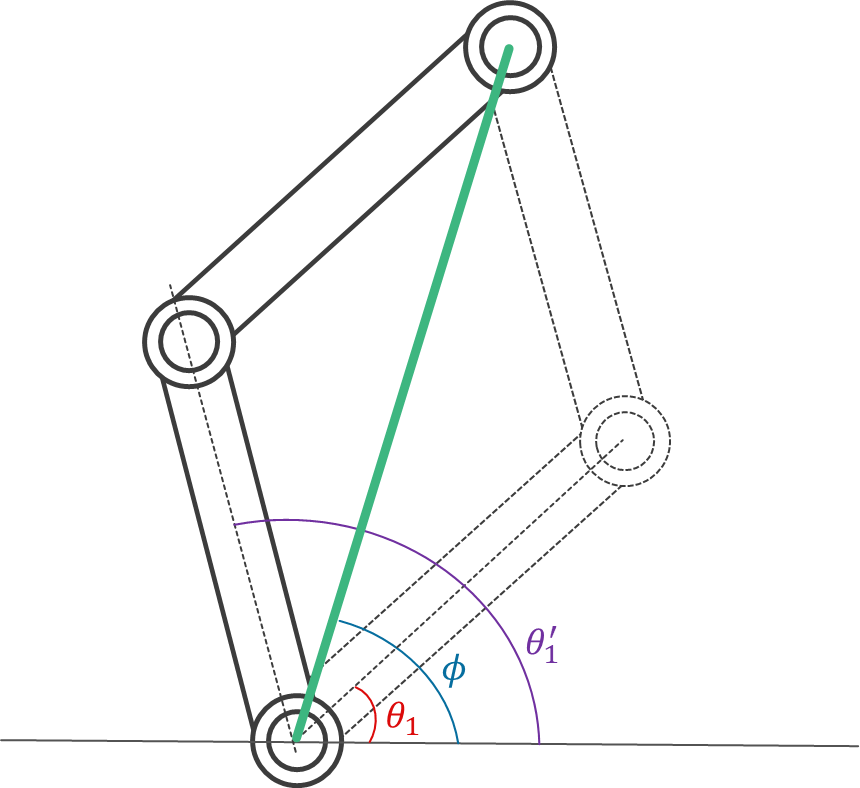
ここで、 $\theta_1$ に注目してみると、プラス·マイナスの2パターンの解が登場することが分かります。
これは、下図のような実際の2リンクのシリアルリンクロボットアームをイメージしてみると分かります。
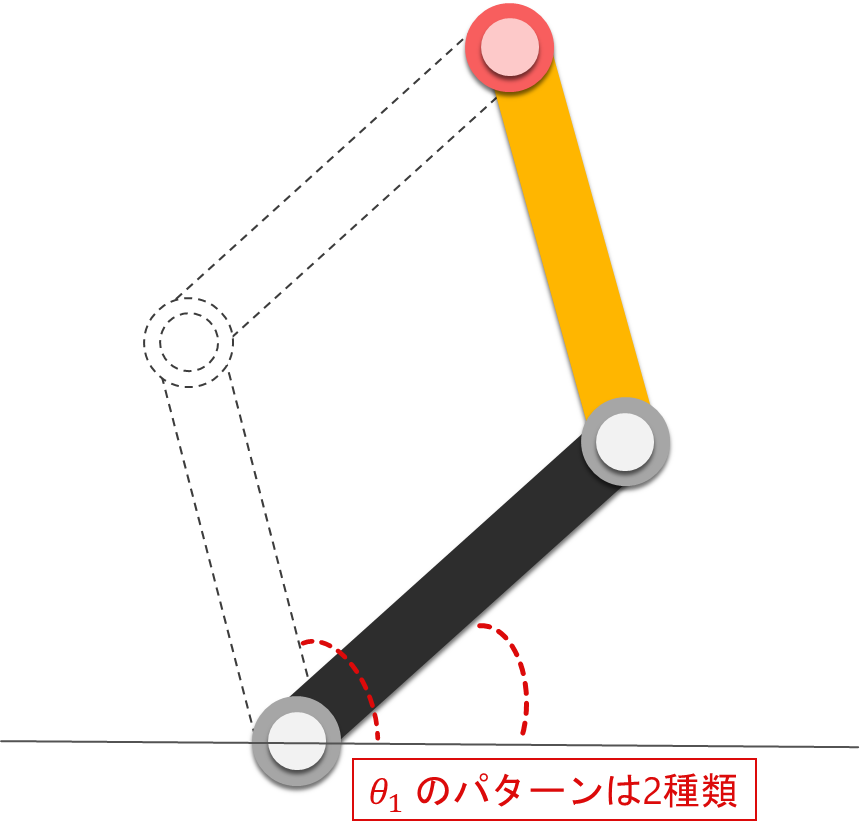
このように
逆運動学には、複数の解が存在する
ということが分かります。
次に $\theta_2$ についても解いていきます。
最初に、式(1)(2)の両辺を2乗します。
\begin{align}
x_{\mathrm{e}}^2 &= (L_1\cos(\theta_1)+L_2\cos(\theta_1+\theta_2))^2\\
&=L_1^2\cos^2(\theta_1)+2L_1\cos(\theta_1)L_2\cos(\theta_1+\theta_2)+L_2^2\cos^2(\theta_1+\theta_2)
 \tag{1'''}
\end{align}
\begin{align}
y_{\mathrm{e}}^2&=(L_1\sin(\theta_1)+L_2\sin(\theta_1+\theta_2))^2 \\
&=L_1^2\sin^2(\theta_1)+2L_1\sin(\theta_1)L_2\sin(\theta_1+\theta_2)+L_2^2\sin^2(\theta_1+\theta_2)
\end{align}
\tag{2'''}
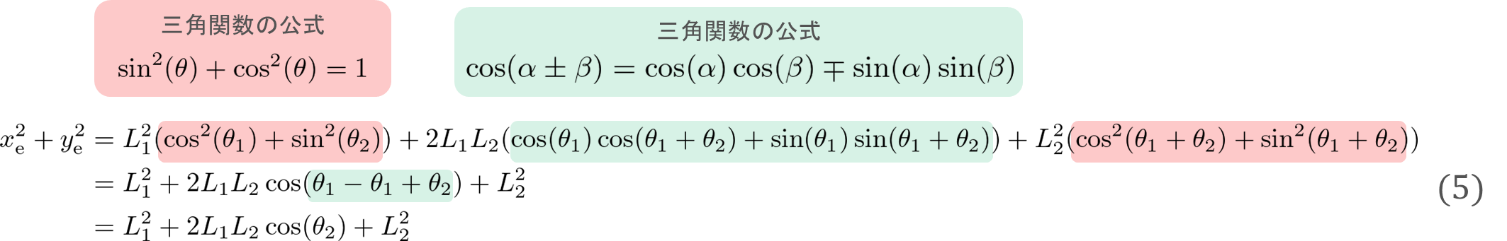
次に、式(1''')と(2''')を足します。
\begin{align}
x_{\mathrm{e}}^2 + y_{\mathrm{e}}^2 &= L_1^2(\cos^2(\theta_1)+\sin^2(\theta_2))+2L_1L_2(\cos(\theta_1)\cos(\theta_1+\theta_2)+\sin(\theta_1)\sin(\theta_1+\theta_2))+L_2^2(\cos^2(\theta_1+\theta_2)+\sin^2(\theta_1+\theta_2)) \\
 &= L_1^2+2L_1L_2\cos(\theta_1-\theta_1+\theta_2)+L_2^2\\
 &= L_1^2+2L_1L_2\cos(\theta_2)+L_2^2\\
\end{align}\tag{5}
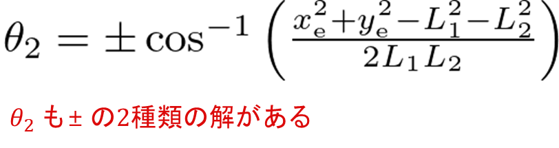
最後に、$\theta_2$ について解きます。
\begin{align}
2L_1L_2\cos(\theta_2) &= x_{\mathrm{e}}^2+y_{\mathrm{e}}^2-L_1^2-L_2^2\\
\cos(\theta_2)&=\frac{x_{\mathrm{e}}^2+y_{\mathrm{e}}^2-L_1^2-L_2^2}{2L_1L_2}\\
\theta_2 &= \pm\cos^{-1}\left(\frac{x_{\mathrm{e}}^2+y_{\mathrm{e}}^2-L_1^2-L_2^2}{2L_1L_2}\right)\tag{6}
\end{align}
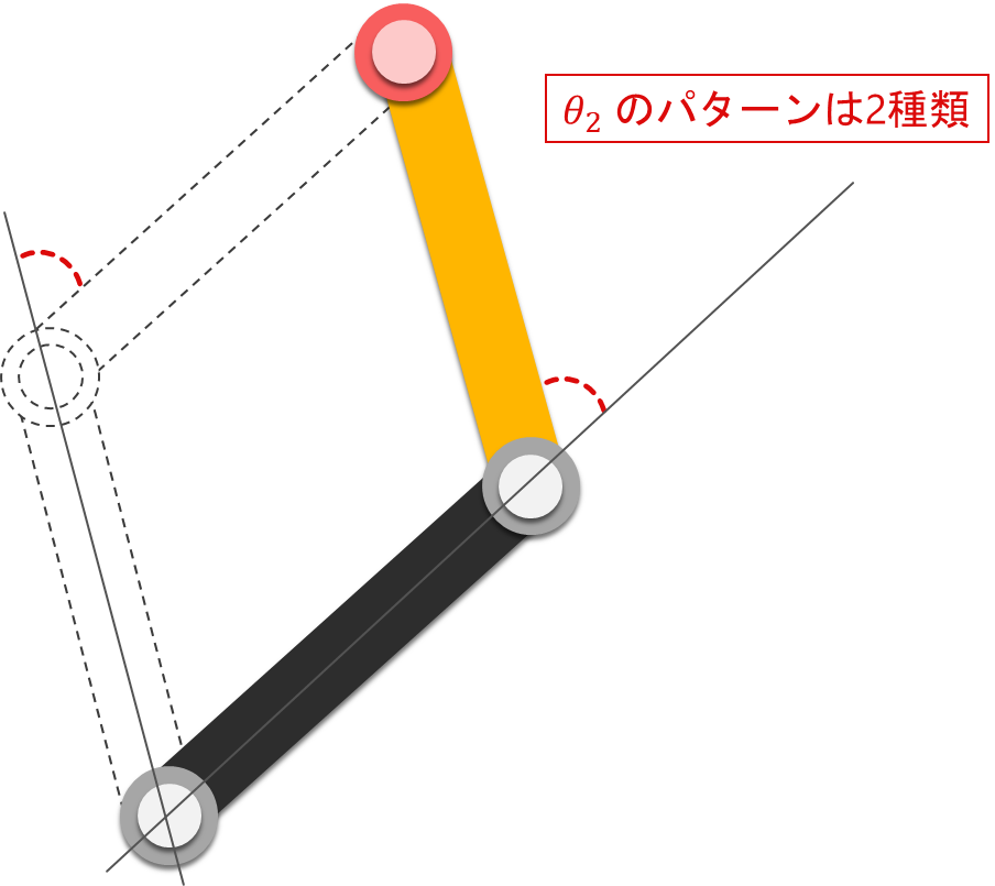
ここで、上式を確認すると $\theta_1$ と同様に、プラス·マイナスの2パターンの解が登場していることが分かります。
最後に、解をまとめると
\begin{align}
\theta_1
&=
\mp\cos^{-1}\left(\frac{x_{\mathrm{e}}^2  + y_{\mathrm{e}}^2 + L_1^2  -L_2^2   }{2L_1 \sqrt{x_{\mathrm{e}}^2+y_{\mathrm{e}}^2}}\right) + \tan^{-1} \left(\frac{ y_{\mathrm{e}} }{ x_{\mathrm{e} }}\right) \\
\theta_2 &= \pm\cos^{-1}\left(\frac{x_{\mathrm{e}}+y_{\mathrm{e}}-L_1-L_2}{2L_1L_2}\right)

\end{align}
となり、これで「各関節の角度 $\theta_1, \theta_2$ 」について解くことができました。
方法2)幾何学的に求める
次は、幾何学的な方法で「各関節の角度 $\theta_1, \theta_2$ 」を求めてみましょう。
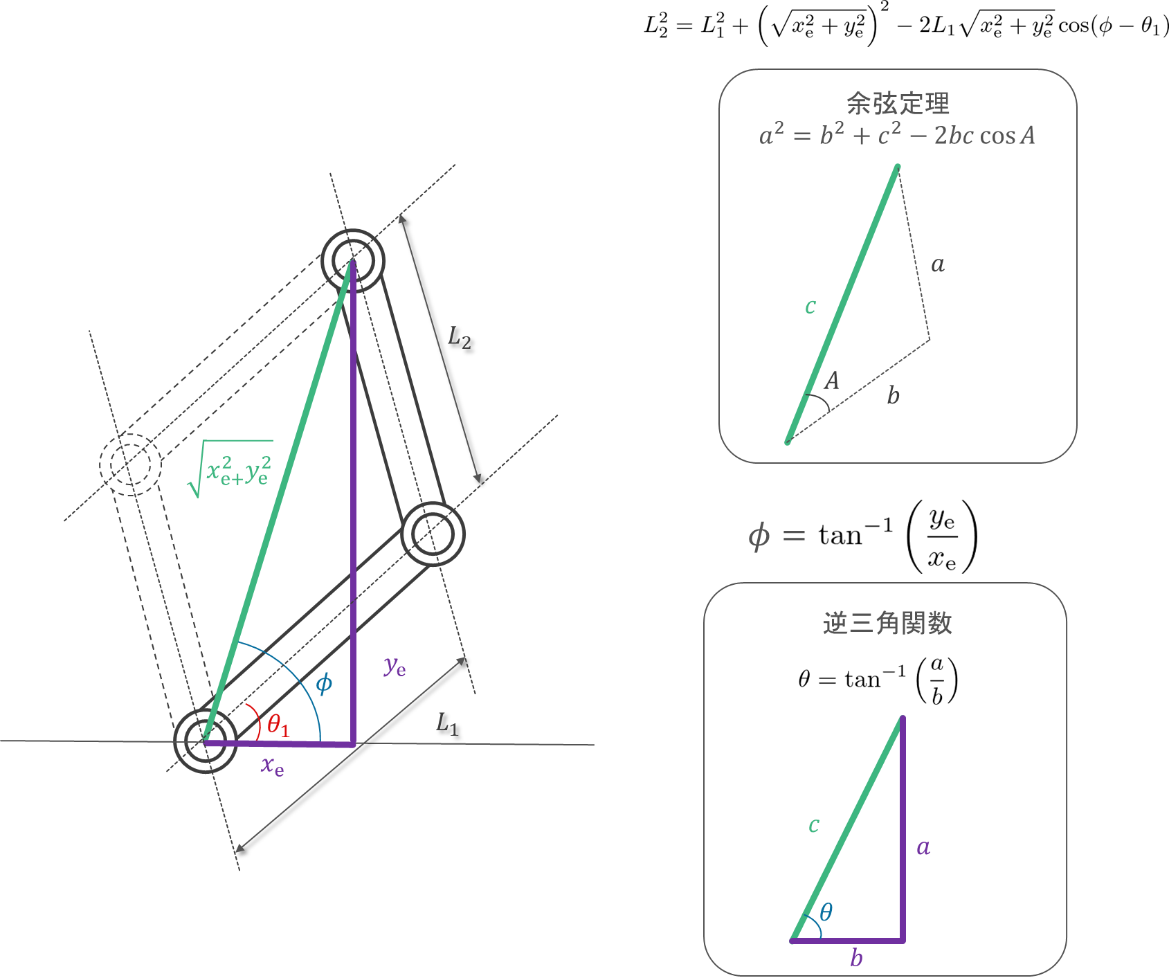
最初に、$\theta_1$ を求めてみましょう。
\begin{align}
L_2^2
&=
L_1^2+\left(\sqrt{x_\mathrm{e}^2 + y_\mathrm{e}^2}\right)^2-2L_1\sqrt{x_\mathrm{e}^2 + y_\mathrm{e}^2}\cos(\phi-\theta_1) \\

L_2^2
&=
L_1^2+x_\mathrm{e}^2 + y_\mathrm{e}^2-2L_1\sqrt{x_\mathrm{e}^2 + y_\mathrm{e}^2}\cos(\phi-\theta_1) \\

L_2^2 - L_1^2 - x_\mathrm{e}^2 - y_\mathrm{e}^2
&=
-2L_1\sqrt{x_\mathrm{e}^2 + y_\mathrm{e}^2}\cos(\phi-\theta_1) \\

\frac{-L_2^2 + L_1^2 + x_\mathrm{e}^2 + y_\mathrm{e}^2}{2L_1\sqrt{x_\mathrm{e}^2 + y_\mathrm{e}^2}}
&=
\cos(\phi-\theta_1) \\

\cos^{-1}\left(\frac{-L_2^2 + L_1^2 + x_\mathrm{e}^2 + y_\mathrm{e}^2}{2L_1\sqrt{x_\mathrm{e}^2 + y_\mathrm{e}^2}}\right)
&=
\phi-\theta_1 \\

\theta_1
&=
\phi-\cos^{-1}\left(\frac{-L_2^2 + L_1^2 + x_\mathrm{e}^2 + y_\mathrm{e}^2}{2L_1\sqrt{x_\mathrm{e}^2 + y_\mathrm{e}^2}}\right)\\

\theta_1
&=
\tan^{-1}\left(\frac{y_\mathrm{e}}{x_\mathrm{e}}\right)-\cos^{-1}\left(\frac{-L_2^2 + L_1^2 + x_\mathrm{e}^2 +y_\mathrm{e}^2}{2L_1\sqrt{x_\mathrm{e}^2 + y_\mathrm{e}^2}}\right) \\

\tag{1}
\end{align}
ここで、1つ目の関節の角度は2パターン存在し、もう一方の関節角度$\theta_1^{\prime}$ は以下式で表すことができます。
\begin{align}
\theta_1^{\prime}
&=
\theta_1+2(\phi-\theta_1) \\

&=
\theta_1+2\phi-2\theta_1 \\

&=
2\phi-\theta_1 \\

\tag{2}

\end{align}
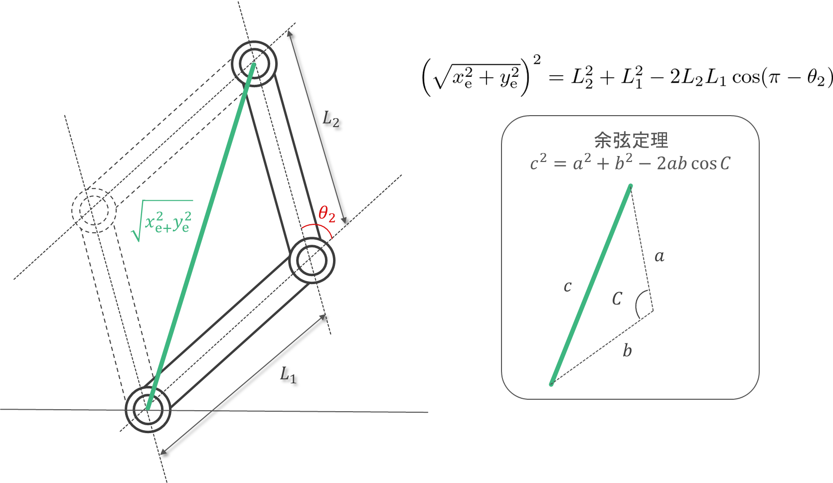
次に、$\theta_2$ についても解いてみましょう。
\begin{align}

\left(\sqrt{x_\mathrm{e}^2+y_\mathrm{e}^2}\right)^2
&=
L_2^2+L_1^2-2L_2L_1\cos(\pi-\theta_2)\\

x_\mathrm{e}^2+y_\mathrm{e}^2
&=
L_2^2+L_1^2-2L_2L_1\cos(\pi-\theta_2)\\

x_\mathrm{e}^2+y_\mathrm{e}^2-L_2^2-L_1^2
&=
-2L_2L_1\cos(\pi-\theta_2)\\

\frac{-x_\mathrm{e}^2-y_\mathrm{e}^2+L_2^2+L_1^2}{2L_2L_1}
&=
\cos(\pi-\theta_2)\\

\cos^{-1}\left(\frac{-x_\mathrm{e}^2-y_\mathrm{e}^2+L_2^2+L_1^2}{2L_2L_1}\right)
&=
\pi-\theta_2 \\

\theta_2
&=
\pi-\cos^{-1}\left(\frac{-x_\mathrm{e}^2-y_\mathrm{e}^2+L_2^2+L_1^2}{2L_2L_1}\right)

\end{align}
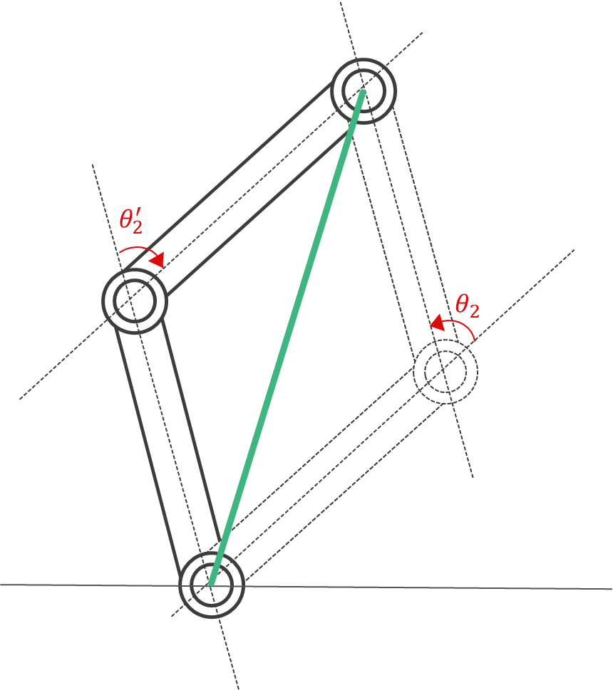
ここで、2つ目の関節の角度も2パターン存在し、もう一方の関節角度$\theta_2^{\prime}$ は以下式で表すことができます。
$\theta_2^{\prime} = -\theta_2$
最後に、解をまとめると
\begin{align}
\theta_1
&=
\phi-\cos^{-1}\left(\frac{-L_2^2 + L_1^2 + x_\mathrm{e}^2 + y_\mathrm{e}^2}{2L_1\sqrt{x_\mathrm{e}^2 + y_\mathrm{e}^2}}\right)\\
\theta_1^{\prime}
&=
2\phi-\theta_1 \\
\\
\theta_2
&=
\pi-\cos^{-1}\left(\frac{-x_\mathrm{e}^2-y_\mathrm{e}^2+L_2^2+L_1^2}{2L_2L_1}\right)\\
\theta_2^{\prime}
&= -\theta_2
\end{align}
となり、これで幾何学的な解法でも「各関節の角度 $\theta_1, \theta_2$ 」について解くことができました。
(方法1)(方法2)に適当な手先座標 $(x_{\mathrm{e}}, x_{\mathrm{e}})$ を代入してみると、 どちらの方法も同じ解が得られることが確認できる と思うので、試してみてください。
コード
ここまでに説明した内容をpythonで記述すると下記コードのようになります。
下記コードを実行すると、下記画像のような2リンクアームが描画されます。
import math
import matplotlib.pyplot as plt
import numpy as np
import matplotlib.patches as pat

def inverse_kinematics_2link(l1, l2, xe, ye):
    """
    2次元平面上の2リンクロボットアームの逆運動学を求める

    Parameters
    ----------
    l1 : float
        リンク1の長さ
    l2 : float
        リンク2の長さ
    xe : float
        手先のx座標
    ye : float
        手先のy座標

    Returns
    -------
    theta1 : float
        リンク1の関節角度(rad)
    theta2 : float
        リンク2の関節角度(rad)
    """
    try:
        # 代数的に求めた逆運動学の式
        theta1 = -math.acos((xe**2 + ye**2 + l1**2 - l2**2)/(2 * l1 * math.sqrt(xe**2 + ye**2))) + math.atan2(ye, xe)
        theta2 = math.acos((xe**2 + ye**2 - l1**2 - l2**2)/(2 * l1 * l2))

        # 幾何学的に求めた逆運動学の式(「幾何学的」な手法を試したい場合は、下記のコメントを外してください)
        # theta1 = math.atan2(ye,xe) - math.acos((-l2**2 + l1**2 + xe**2 + ye**2)/(2 * l1 * math.sqrt(xe**2 + ye**2)))
        # theta2 = math.pi - math.acos((-xe**2 - ye**2 + l2**2 + l1**2)/(2 * l2* l1))
    except: # 解が存在しない(xe, ye)を入力した場合、Noneを出力
        theta1 = None
        theta2 = None
    return theta1, theta2

##### ここを変更すると結果が変わります #######
# 各リンクの長さ
l1 = 2
l2 = 2

# 手先の座標
xe = -1.0
ye = 3.0
############################################

theta1, theta2 = inverse_kinematics_2link(l1, l2, xe, ye)

############# 以下描画用 ###################################

# 描画には各リンクの先端の座標が必要なので、求めたtheta1, theta2を使って順運動学を解く(描画しないなら不要)
# 同次変換行列(順運動学)← 「同次変換行列による順運動学」の記事はこちら https://qiita.com/akinami/items/9e65389929cedb1c9551
def make_homogeneous_transformation_matrix(link_length, theta):
    """
    2次元平面における同次変換行列を求める

    Parameters
    ----------
    link_length : float
        リンクの長さ
    theta : float
        回転角度(rad)

    Returns
    -------
    T : numpy.ndarray
        同次変換行列
    """
    return np.array([[np.cos(theta), -np.sin(theta), link_length*np.cos(theta)],
                     [np.sin(theta),  np.cos(theta), link_length*np.sin(theta)],
                     [            0,              0,                        1]])


def draw_link_coordinate(ax, matrix, axes_length):
    """
    2次元の変換行列より単位ベクトルを描画

    Parameters
    ----------
    ax : matplotlib.axes._axes.Axes
        描画用
    matrix: numpy.array
        2次元の変換行列
    axes_length : float
        各軸方向の単位ベクトルの長さ

    Returns
    -------
    なし
    """
    # x方向の単位ベクトル
    unit_x = matrix@np.array([[axes_length],
                              [0],
                              [1]])

    # y方向の単位ベクトル
    unit_y = matrix@np.array([[0],
                              [axes_length],
                              [1]])

    x = matrix[0][2]; y = matrix[1][2]

    # x方向の単位ベクトルを描画
    ax.plot([x, unit_x[0][0]], [y, unit_x[1][0]], "o-", color="red", ms=2)
    # y方向の単位ベクトル
    ax.plot([x, unit_y[0][0]], [y, unit_y[1][0]], "o-", color="green", ms=2)

fig = plt.figure(figsize=(5,5))
ax = fig.add_subplot(1,1,1)

# 角度が求められたら描画
if (theta1 is not None) and (theta2 is not None):
    x1, y1 = 0, 0
    H12 = make_homogeneous_transformation_matrix(l1, theta1)
    H2e = make_homogeneous_transformation_matrix(l2, theta2)
    H12e = H12@H2e

    o2 = H12@np.array([[x1],
                    [y1],
                    [1]])
    x2, y2 = o2[0][0], o2[1][0]

    oe = H12e@np.array([[x1],
                        [y1],
                        [1]])

    #アームの駆動範囲の円(真円)
    circle1 = pat.Circle(xy = (x1, y1), radius= l1+l2, color="blue", alpha=0.1)
    ax.add_patch(circle1)

    plt.xlim(-(l1+l2),(l1+l2))
    plt.ylim(-(l1+l2),(l1+l2))

    axes_length = (l1+l2)*0.1
    draw_link_coordinate(ax, np.array([[1, 0, 0],
                                    [0, 1, 0],
                                    [0, 0, 1]]), axes_length) # 座標系1の描画
    draw_link_coordinate(ax, H12, axes_length) # 座標系2の描画
    ax.plot([x1, x2], [y1, y2], color="tomato") # link1の描画
    ax.plot([x2, xe], [y2, ye], color="lightgreen") # link2の描画
    plt.show()
    print("theta1:",math.degrees(theta1))
    print("theta2:",math.degrees(theta2))
else:
    print("手先の座標が範囲外です。")
インタラクティブに動かす(おまけ)
以下コードを実行すると、以下gif画像のようにインタラクティブに手先の座標を変更することができます。
インタラクティブに結果が変わる様子を確認することで、逆運動学の理解が更に深まると思うので、よろしければこちらのコードも試してみてください。
google colaboratory上では、ラグが発生するため上記動画よりも遅れて描画される可能性があります。
import numpy as np
import matplotlib.pyplot as plt
import ipywidgets
import math
import matplotlib.patches as pat
%matplotlib inline

def inverse_kinematics_2link(l1, l2, xe, ye):
    """
    2次元平面上の2リンクロボットアームの逆運動学を求める

    Parameters
    ----------
    l1 : float
        リンク1の長さ
    l2 : float
        リンク2の長さ
    xe : float
        手先のx座標
    ye : float
        手先のy座標

    Returns
    -------
    theta1 : float
        リンク1の関節角度(rad)
    theta2 : float
        リンク2の関節角度(rad)
    """
    try:
        # 代数的に求めた逆運動学の式
        theta1 = -math.acos((xe**2 + ye**2 + l1**2 - l2**2)/(2 * l1 * math.sqrt(xe**2 + ye**2))) + math.atan2(ye, xe)
        theta2 = math.acos((xe**2 + ye**2 - l1**2 - l2**2)/(2 * l1 * l2))

        # 幾何学的に求めた逆運動学の式(「幾何学的」な手法を試したい場合は、下記のコメントを外してください)
        # theta1 = math.atan2(ye,xe) - math.acos((-l2**2 + l1**2 + xe**2 + ye**2)/(2 * l1 * math.sqrt(xe**2 + ye**2)))
        # theta2 = math.pi - math.acos((-xe**2 - ye**2 + l2**2 + l1**2)/(2 * l2* l1))
    except: # 解が存在しない(xe, ye)を入力した場合、Noneを出力
        theta1 = None
        theta2 = None
    return theta1, theta2

# 描画には各リンクの先端の座標が必要なので、逆運動学によって求めたtheta1, theta2を使って順運動学を解く(描画しないなら不要)
# 同次変換行列(順運動学)← 「同次変換行列による順運動学」の記事はこちら https://qiita.com/akinami/items/9e65389929cedb1c9551
def make_homogeneous_transformation_matrix(link_length, theta):
    """
    2次元平面における同次変換行列を求める

    Parameters
    ----------
    link_length : float
        リンクの長さ
    theta : float
        回転角度(rad)

    Returns
    -------
    T : numpy.ndarray
        同次変換行列
    """
    return np.array([[np.cos(theta), -np.sin(theta), link_length*np.cos(theta)],
                     [np.sin(theta),  np.cos(theta), link_length*np.sin(theta)],
                     [            0,              0,                        1]])

def draw_link_coordinate(ax, matrix, axes_length):
    """
    2次元の変換行列より単位ベクトルを描画

    Parameters
    ----------
    ax : matplotlib.axes._axes.Axes
        描画用
    matrix: numpy.array
        2次元の変換行列
    axes_length : float
        各軸方向の単位ベクトルの長さ

    Returns
    -------
    なし
    """
    # x方向の単位ベクトル
    unit_x = matrix@np.array([[axes_length],
                              [0],
                              [1]])

    # y方向の単位ベクトル
    unit_y = matrix@np.array([[0],
                              [axes_length],
                              [1]])

    x = matrix[0][2]; y = matrix[1][2]

    # x方向の単位ベクトルを描画
    ax.plot([x, unit_x[0][0]], [y, unit_x[1][0]], "o-", color="red", ms=2)
    # y方向の単位ベクトル
    ax.plot([x, unit_y[0][0]], [y, unit_y[1][0]], "o-", color="green", ms=2)

def generate_vbox_text_widget(l1, l2):
    """
    text widgetsを2個作成 -> Vboxに格納して縦に並べる(範囲は-l1-l2〜l1+l2)

    Parameters
    ----------
    l1 : float
        リンク1の長さ
    l2 : float
        リンク2の長さ

    Returns
    -------
    vox_text_widgets : ipywidgets.widgets.widget_box.VBox
        text widgetsをnum個,縦に並べたVBox
    """
    text_widgets = []
    for i in range(2):
      text_widgets.append(ipywidgets.FloatText(min=-l1-l2, max=l1+l2))
    vox_text_widgets = ipywidgets.VBox(text_widgets)
    return vox_text_widgets

def generate_vbox_slider_widget(l1, l2):
    """
    slider widgetsを2個作成 -> Vboxに格納して縦に並べる.(範囲は-l1-l2〜l1+l2)

    Parameters
    ----------
    l1 : float
        リンク1の長さ
    l2 : float
        リンク2の長さ

    Returns
    -------
    vox_slider_widgets : ipywidgets.widgets.widget_box.VBox
        slider widgetsをnum個,縦に並べたVBox
    """
    slider_widgets = []

    slider_widgets.append(ipywidgets.FloatSlider(value=0.0, min=-l1-l2, max=l1+l2, description = "xe:", disabled=False))
    slider_widgets.append(ipywidgets.FloatSlider(value=0.0, min=-l1-l2, max=l1+l2, description = "ye:", disabled=False))
    vox_slider_widgets = ipywidgets.VBox(slider_widgets)
    return vox_slider_widgets


def link_slider_and_text(box1, box2):
    """
    Box内の複数のwidetを連携させる(二つのbox内のwidgetの数が同じである必要あり)

    Parameters
    ----------
    box1 : ipywidgets.widgets.widget_box.VBox
        boxの名前
    box2 : ipywidgets.widgets.widget_box.VBox
        boxの名前
    link_num : int
        linkの数
    """
    for i in range(2):
      ipywidgets.link((box1.children[i], 'value'), (box2.children[i], 'value'))

def draw_interactive(l1, l2):
    """
    結果をアニメーションで表示
    Parameters
    ----------
    link_num : int
        linkの数
    """
    # slider widgetを作成
    posture_sliders = generate_vbox_slider_widget(l1, l2)
    # text widgetを作成
    posture_texts = generate_vbox_text_widget(l1, l2)

    # slider widget と posture widget を横に並べる
    slider_and_text = ipywidgets.Box([posture_sliders, posture_texts])

    # slider wiget と text widget を連携
    link_slider_and_text(posture_sliders, posture_texts)

    # リセットボタン
    reset_button = ipywidgets.Button(description = "Reset")
    # 姿勢のリセットボタン
    def reset_values(button):
        for i in range(2):
            posture_sliders.children[i].value = 0.0
    reset_button.on_click(reset_values)

    # main文にslider widgetsの値を渡す
    params = {}
    for i in range(2):
        params[str(i)] = posture_sliders.children[i]
    final_widgets = ipywidgets.interactive_output(main, params)

    display(slider_and_text, reset_button, final_widgets)

# 各リンクの長さ
l1 = 2.0
l2 = 2.0
def main(*args, **kwargs):

    params = kwargs
    fig = plt.figure(figsize=(5,5))
    ax = fig.add_subplot(1,1,1)
    ################ ここから逆運動学にの処理(メイン部分) #############################

    # 手先位置(可変)
    xe = params["0"]
    ye = params["1"]

    theta1, theta2 = inverse_kinematics_2link(l1, l2, xe, ye)

    ####################### 以下描画 ################################################
    if (theta1 is not None) and (theta2 is not None):
        x1, y1 = 0, 0
        H12 = make_homogeneous_transformation_matrix(l1, theta1)
        H2e = make_homogeneous_transformation_matrix(l2, theta2)
        H12e = H12@H2e

        o2 = H12@np.array([[x1],
                        [y1],
                        [1]])
        x2, y2 = o2[0][0], o2[1][0]

        oe = H12e@np.array([[x1],
                            [y1],
                            [1]])
        xe, ye = oe[0][0], oe[1][0]

        #アームの駆動範囲の円(真円)
        circle1 = pat.Circle(xy = (x1, y1), radius= l1+l2, color="blue", alpha=0.1)
        ax.add_patch(circle1)

        plt.xlim(-(l1+l2),(l1+l2))
        plt.ylim(-(l1+l2),(l1+l2))

        axes_length = (l1+l2)*0.1
        draw_link_coordinate(ax, np.array([[1, 0, 0],
                                        [0, 1, 0],
                                        [0, 0, 1]]), axes_length) # 座標系1の描画
        draw_link_coordinate(ax, H12, axes_length) # 座標系2の描画
        ax.plot([x1, x2], [y1, y2], color="tomato") # link1の描画
        ax.plot([x2, xe], [y2, ye], color="lightgreen") # link2の描画
        plt.grid()
        plt.show()
        print("theta1:",math.degrees(theta1))
        print("theta2:",math.degrees(theta2))
    else:
        print("手先の座標が範囲外です。")

draw_interactive(l1, l2)
さいごに
ここまでで、 解析的に逆運動学を解く方法を紹介しました。
このように、解析的解法では一度数式を求めてしまえば、以降は手先の位置を代入するだけで一瞬で各関節の角度を求めることができます(高速&高精度)
一方で、式を見てもらえればわかる通り、2軸のシンプルな機構であっても数式が割と複雑になことがわかると思います。
これが6軸、7軸のような多軸のロボットになると、数式が更に複雑になります。
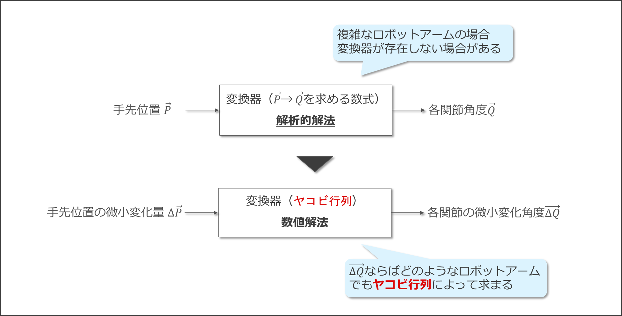
今回解説した「手先位置$\vec{P}$」から「各関節角度$\vec{Q}$」を求める数式を「変換器」とみなすと、ロボットの構成によってはこの変換器が存在しない場合がある、すなわち解析的な方法では逆運動学を解くことができない場合があります。

このような解析的解法のデメリットを解決する手法に数値解法が存在します。
数値解法は、「手先位置の微小変化量$\Delta\vec{P}$」から「各関節の微小変化角度$\Delta \vec{Q}$」を求める変換器であるヤコビ行列を用いることで、各関節角度を少しずつ動かしていくことで、近似的な解を求める手法です。
数値解法は、解析的解法と比較すると軸数の多いロボットでも数式が複雑にならないというメリットが存在します。
一方で、数値解法では近似解を求めるため精度が落ちることや、繰り返し計算をすることにより計算時間がかかることがデメリットとして挙げられます。
解析的解法と数値解法のメリット·デメリットは下に示すように逆の関係になっていることがわかります。
そのため、状況によって解析的解法と数値解法を使い分けるとよいと思います
解析的解法
メリット:一度数式を求めれば、一瞬で解が求まる(高速)。精度が高い
デメリット:アームが複雑になると数式も複雑になる(解が求められない場合もある)
数値解法
メリット:アームが複雑になっても数式が複雑にならない
デメリット:繰り返し計算により解を求めるため計算速度は遅い。近似解であるため精度が低い
次回は この「数値解法による逆運動学」について解説します。
以上で,「解析的解法による逆運動学」の説明は終わりになります.ロボティクスに興味のある方のお役に少しでも立てたら幸いです.