[Python]状態空間モデルの同定

目的

状態空間モデルのシステム同定方法の確認を行った為、確認に用いたPythonスクリプトを紹介する。

学習用データ作成のためのモデルおよび学習するモデル。

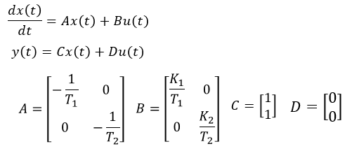
学習用データ作成のためのモデルおよび学習するモデルは以下のような２入力１出力の１次遅れ系とした。
・状態量x1が入力u1に対して一時遅れ系
・状態量x2が入力u2に対して一時遅れ系
・出力yは状態量x1,x2の合計

システム同定方法

定常ゲインK1,K2および時定数T1,T2を下式で最適化する。

学習用データおよびシステム同定結果

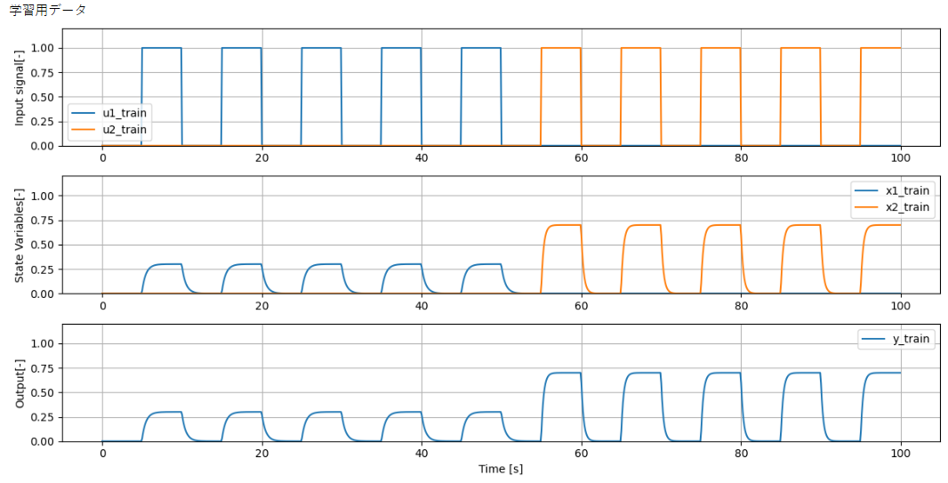
学習用データ step信号、検証用データ chirp信号

学習用データ(入力信号 Step信号)
学習用データu1とu2が相関をもつと、正しく同定できない（出力は一致するが状態量が一致せず）為、u1とu2がステップするタイミングを分けている。

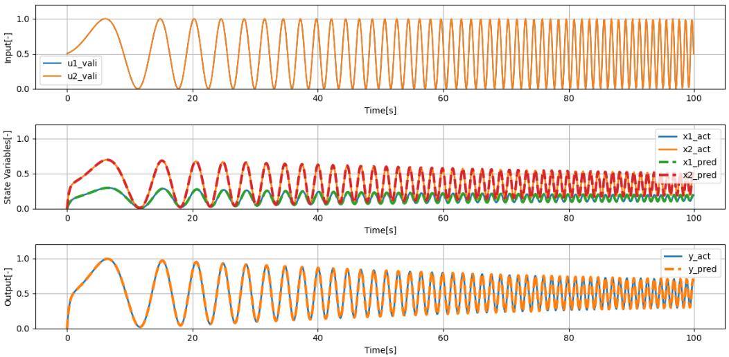
検証結果（入力信号 Charp信号）
出力および状態量が一致しているため問題なく同定できていると判断する。

学習用データ 白色ノイズ、検証用データ chirp信号

学習用データ(入力信号 白色ノイズ)
白色ノイズはもともとu1とu2の相関はないので、相関を気にせずにに同定可能。

検証結果
出力および状態量が一致しているため問題なく同定できていると判断する。

スクリプト

d14a_SS_Identification.py

import numpy as np
import matplotlib.pyplot as plt
from control.matlab import *
from scipy.optimize import minimize

#時定数と定常ゲインからシステムを作成する
def get_sys(T1, T2, K1, K2):
    # システム行列(出力は各一時遅れ系２ケの合計)
    A = np.array([[-1/T1, 0], [0, -1/T2]])
    B = np.array([[K1/T1, 0], [0, K2/T2]])
    C = np.array([[1, 1]])
    D = np.array([[0, 0]])

    return ss(A, B, C, D);

#-------------学習用データを作成するためのモデル--------------
# 状態空間モデル
sys_act = get_sys(T1=0.5, T2=0.3, K1=0.3, K2=0.7)

#学習用データと検証用データを作成するための入力信号の種類・・・予測精度に大きな影響がある
#1:Step信号、2:Chirp信号、3:白色ノイズ
train_data_type = 3
vali_data_type = 2

#学習データおよび検証用データを作成するための入力信号
duration = 100  # 信号の継続時間 (秒)
sampling_rate = 10  # サンプリングレート (Hz)

#信号作成用の関数
def make_signal(step_signal_type):
    if step_signal_type ==1: #---Step信号---
        step_time = duration/20 #ステップするタイミングをdurationの1/20毎とする
        u = np.zeros_like(time_org)
        for i in range(len(time_org)):
            if (i // int(step_time * sampling_rate)) % 2 == 1:
                u[i] = 1
        return u
    elif step_signal_type ==2: #---Chirp信号---
        frequency_start = 0.01  # チャープ信号の開始周波数 (Hz)
        frequency_end = 1 # チャープ信号の終了周波数 (Hz)
        u = np.sin(2 * np.pi * np.cumsum(np.linspace(frequency_start, frequency_end, len(time_org)) / sampling_rate)) / 2 + 0.5
        return u
    else: #---白色ノイズ---
        A = 1.0    # 振幅
        u = 1*A*(np.random.rand(round(sampling_rate*duration)))
        return u

# 時間軸の作成
time_org = np.linspace(0, duration, int(sampling_rate * duration), endpoint=False)

#学習用入力信号の作成
if train_data_type == 3:
    u1 =  make_signal(train_data_type)
    u2 =  make_signal(train_data_type)
else:
    u1 =  make_signal(train_data_type)
    half_length = len(u1) // 2
    u1[half_length:] = 0

    u2 =  make_signal(train_data_type)
    half_length = len(u2) // 2
    u2[:half_length] = 0

U_train = np.vstack([u1, u2]).T

#-----------------lsimで応答計算-------------------
y_train, t_temp, X_train = lsim(sys_act, U=U_train, T=time_org)

#-----------------Xとyの時系列グラフを表示-----------------
plt.figure(figsize=(12, 6))
#plot U
plt.subplot(3, 1, 1)
plt.plot(time_org, U_train, label=['u1_train','u2_train'])
plt.ylabel('Input signal[-]')
plt.ylim([0,1.2])
plt.grid(True)
plt.legend()

# Plot X
plt.subplot(3, 1, 2)
plt.plot(time_org, X_train, label=['x1_train','x2_train'])
plt.ylabel('State Variables[-]')
plt.ylim([0,1.2])
plt.grid(True)
plt.legend()

# Plot y
plt.subplot(3, 1, 3)
plt.plot(time_org, y_train, label='y_train')
plt.xlabel('Time [s]')
plt.ylabel('Output[-]')
plt.ylim([0,1.2])
plt.grid(True)
plt.legend()

plt.tight_layout()
plt.show()

#-------------システム同定---------------
# 目的関数の定義
global count
count = 0
def objective(params, U_train, time_org, y_train):
    global count
    count = count + 1
    sys = get_sys(params[0],params[1],params[2],params[3])
    y_pred, _, _ = lsim(sys, U=U_train, T=time_org)
    sse = np.sum((y_train - y_pred)**2)
    if count % 100 == 1:
        print('count:',count,' sse:',round(sse, 3))
    return sse

# 初期パラメータの設定
initial_params = np.random.rand(4)

# 最適化
result = minimize(objective, initial_params, args=(U_train, time_org, y_train), method='Nelder-Mead')

# 最適化されたパラメータを使用してモデルを再構築
T1_pred = result.x[0]
T2_pred = result.x[1]
K1_pred = result.x[2]
K2_pred = result.x[3]
sys_pred = get_sys(T1_pred, T2_pred, K1_pred, K2_pred)

print('T1_pred ', round(T1_pred,3), ', T2_pred:', round(T2_pred), ', K1_pred:', round(K1_pred,3) , ', K2_pred:', round(K2_pred,3) )

#検証用入力信号の作成
u1 = make_signal(vali_data_type)
#u2 = np.zeros_like(time_org)
u2 = make_signal(vali_data_type)
U_vali = np.vstack([u1, u2]).T

# オリジナルモデルと最適化されたモデルの応答計算
y_act, _, X_act = lsim(sys_act, U=U_vali, T=time_org)
y_pred, _, X_pred = lsim(sys_pred, U=U_vali, T=time_org)

# 結果のプロット
plt.figure(figsize=(12, 6))

# Plot original and identified system outputs
# Plot input signals
plt.subplot(3, 1, 1)
plt.plot(time_org, U_vali, label=['u1_vali','u2_vali'])
plt.xlabel('Time[s]')
plt.ylabel('Input[-]')
plt.legend()
plt.ylim([0,1.2])
plt.grid(True)

plt.subplot(3, 1, 2)
plt.plot(time_org, X_act, label=['x1_act','x2_act'],linewidth=2)
plt.plot(time_org, X_pred, label=['x1_pred','x2_pred'], linestyle='--',linewidth=3)
plt.xlabel('Time[s]')
plt.ylabel('State Variables[-]')
plt.legend()
plt.ylim([0,1.2])
plt.grid(True)

plt.subplot(3, 1, 3)
plt.plot(time_org, y_act, label='y_act',linewidth=2)
plt.plot(time_org, y_pred, label='y_pred', linestyle='--',linewidth=3)
plt.xlabel('Time[s]')
plt.ylabel('Output[-]')
plt.legend()
plt.ylim([0,1.2])
plt.grid(True)


plt.tight_layout()
plt.show()